Open-loop system

See also problem

Problemè 1

A unity feedback system has transfer function

$$G(s)=\frac{K}{s(s^2+4s+13)}$$

1.a

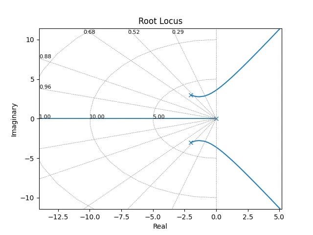
Plot the root locus for this problem

We need to find the poles and zeros of the open-loop transfer function $G(s)$. The poles are given by the roots of the denominator polynomial:

$$s(s^2+4s+13)=0⟹s=0,-2\pm 3j$$

And the following code to draw the plot:

import matplotlib.pyplot as plt
import control as ctl
 
numerator = [1]
denominator = [1, 4, 13, 0]
G_s = ctl.TransferFunction(numerator, denominator)
rlist, klist = ctl.root_locus(G_s, Plot=True, grid=True)
 
# Show the plot
plt.show()

1.b

Find the value of $K$ that gives a damping ration of 0.2588

K is approximately $10.000$.

The following code is used:

# Find the gain K for a damping ratio of 0.2588
K_range = np.linspace(0, 10, 1000)
for K in K_range:
  poles = np.roots(G.den[0][0] + K * G.num[0][0])
  zeta_actual = -np.cos(np.angle(poles[0]))
  if np.abs(zeta_actual - zeta) < 0.001:
    break
 
# Print the gain value
print(f'The gain K for a damping ratio of 0.2588 is approximately: {K:.3f}')

1.c

Find the location of the roots for the value of $K$ found in 1.b

With $K=10$, the poles are [-1.5+2.78388218j -1.5-2.78388218j -1. +0.j ].

The code is:

K = 10
print(np.roots([1, 4, 13, K]))

1.d

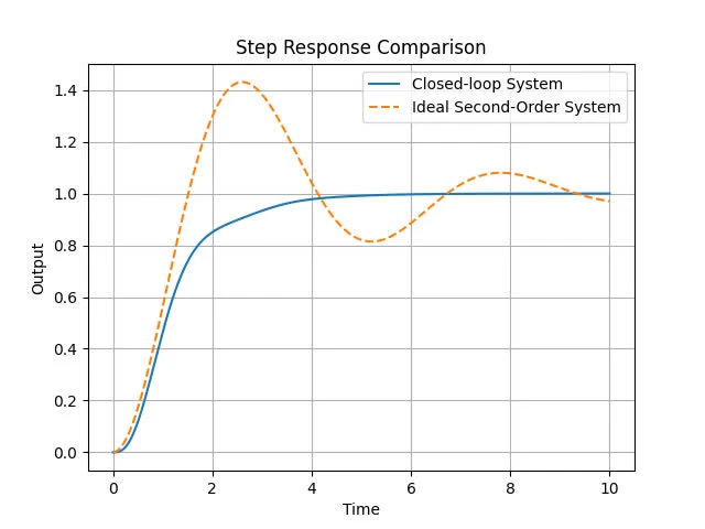
Plot the step response of your closed-loop system, along with the step response of an ideal second order system with damping ratio 0.2588 and poles that correspond to the two poles with imaginary parts.

Here is the code for that:

# Extract the imaginary part of the complex poles
wn = np.abs(poles[0].imag)
 
# Create the closed-loop transfer function with the found gain K
G_cl = ctl.feedback(K * G, 1)
 
# Create an ideal second-order system with the same damping ratio and natural frequency
G_ideal = ctl.tf([wn**2], [1, 2 * zeta * wn, wn**2])
 
# Generate time vector for simulation
t = np.linspace(0, 10, 1000)
 
# Simulate the step response of the closed-loop system and the ideal system
_, y_cl = ctl.step_response(G_cl, t)
_, y_ideal = ctl.step_response(G_ideal, t)
 
# Plot the step responses
plt.figure()
plt.plot(t, y_cl, label='Closed-loop System')
plt.plot(t, y_ideal, '--', label='Ideal Second-Order System')
plt.xlabel('Time')
plt.ylabel('Output')
plt.title('Step Response Comparison')
plt.legend()
plt.grid()
plt.show()

1.e

Find the value of K that leads to a marginally stable system.

The characteristic equation is given by:

$$1+G(s)=0$$

or

$$s^3+4s^2+13s+K=0$$

Let’s setup the Routh-Hurwitz table:

$s^3$	1	13
$s^2$	4	K
$s^1$	$b=13-\frac{K}{4}$	0
$s^0$	K	-

For marginal stability, the system must have poles on the imaginary axis. This occurs when the first element of any row in the Routh array is zero.

Let $b=0$, then $13-\frac{K}{4}=0⟹K=52$.

Therefore, the system is marginally stable for $K=52$. This is the critical gain $K_{cr}$. For $K<52$, all elements in the first column of the Routh array are positive, indicating stability. For $K>52$, there is a sign change in the first column, indicating instability

For frequency oscillation at marginal stability, solve characteristic equation for $s$ with $K=52$:

$$(s^2+4)(s+13)=0$$

imaginary roots are $\pm 2j$, thus frequency of oscillation is $2$ rad/s.

---

Problemè 2

Consider the open-loop system

$$G(s)=\frac{(s+10)}{(s+1)(s+2)(s+12)}$$

2.a

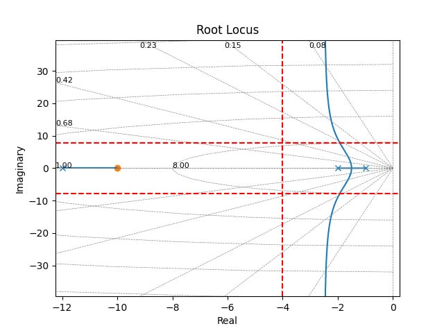
Suppose that design specifications are that the $\%OS$ is 20% and the settling time is 1 second. Use the root-locus approach to design a PD controller for this system.

Given $\%OS$ is 20% and settling time is 1 second, we can find $\zeta$, $\sigma$, ${\omega }_n$ as:

$$\begin{array}{rl}\zeta & =-\ln (\%OS/100)/\sqrt{{\pi }^2+{\ln }^2(\%OS/100)}\approx 0.456\\ \sigma & =\frac{4}{\zeta T_s}\approx 8.77\\ {\omega }_n& =19.24\end{array}$$

The code to find:

import numpy as np
import matplotlib.pyplot as plt
import control as ctl
 
# Desired specifications
OS = 0.20  # 20% overshoot
Ts = 1  # 1 second settling time
 
# Calculations for desired pole locations
zeta = -np.log(OS) / np.sqrt(np.pi**2 + np.log(OS) ** 2)  # damping ratio
sigma = -4 / (zeta * Ts)  # real part of poles
wd = sigma / zeta  # imaginary part of poles
 
print(zeta, sigma, wd)

So desired dominant poles are:

$$s_{1,2}=-\zeta {\omega }_n\pm j{\omega }_n\sqrt{1-{\zeta }^2}=-4\pm 7.66j$$

Propose a PD controller $D(s)=K(s+z)$ where $K$ is the gain and $z$ is the zero introduced by the PD controller.

The code can be found here