Joint-control open-loop system

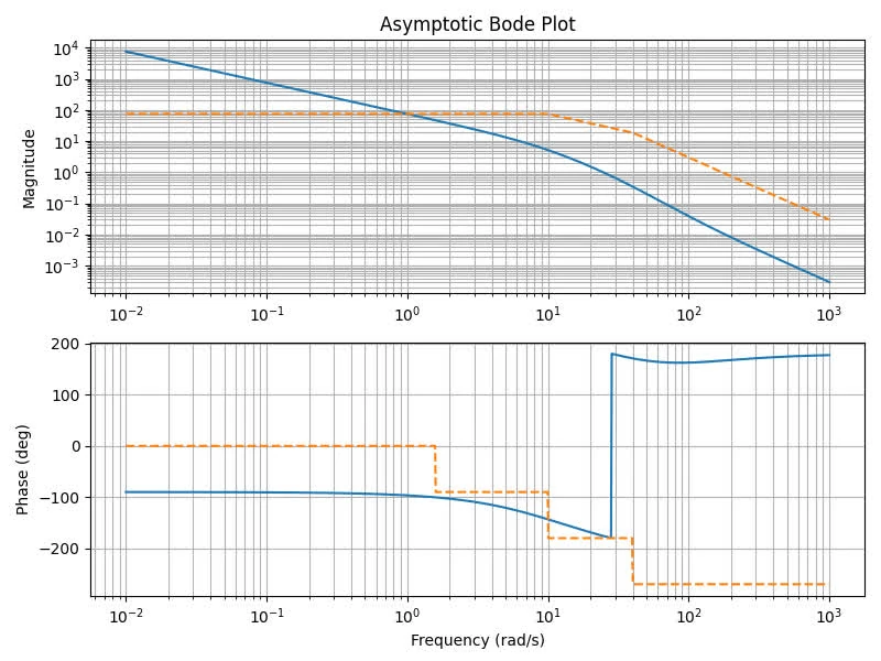
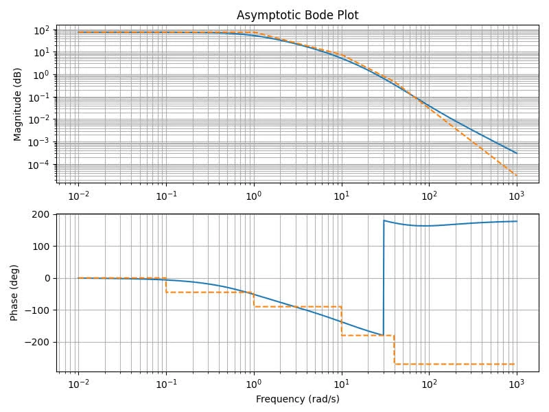
See also problem

Problemè 1

A robot arm has a joint-control open-loop transfer function

$$G(s) = \frac{300(s+100)}{s(s+10)(s+40)}$$

1.a

Plot the asymptotic approximation of the Bode plot

The code can be found in p1a.py

1.b

Repeat this with the pole at 0 and the denominator replaced by a pole at -1

The code can be found in p1b.py

1.c

For the system above, estimate the bandwidth using only the asymptotic approximation

The corner frequency are at 1, 10, 40 rad/s given the poles.

Given the dominant pole is at -1, at 1 rad/s the gain starts dropping at -20 db/Decade.

Therefore, the frequency needs to increase by a factor of $10^{\frac{3}{20}} \approx 1.41 \text{ rad s}$

1.d

Use MATLAB to find the bandwidth of the system in (b). Why is the result different than your answer in c?

The following is the code for finding the bandwidth of the system

% Define the transfer function
num = 300 * [1 100];
den = conv([1 1], conv([1 10], [1 40]));
G = tf(num, den);
 
% Generate frequency vector (in rad/s)
w = logspace(-2, 3, 1000);
 
% Compute magnitude and phase
[mag, phase, w] = bode(G, w);
 
% Asymptotic magnitude approximation
asymp_mag = zeros(size(w));
asymp_mag(w < 1) = 300 * 100 / (1 * 10 * 40);  % DC gain
asymp_mag(w >= 1 & w < 10) = 300 * 100 ./ (w(w >= 1 & w < 10) * 10 * 40);  % -20 dB/dec slope
asymp_mag(w >= 10 & w < 40) = 300 * 100 ./ (w(w >= 10 & w < 40).^2 * 40);  % -40 dB/dec slope
asymp_mag(w >= 40) = 300 * 100 ./ (w(w >= 40).^3);  % -60 dB/dec slope
 
% Asymptotic phase approximation
asymp_phase = zeros(size(w));
asymp_phase(w < 0.1) = 0;  % 0 deg
asymp_phase(w >= 0.1 & w < 1) = -45;  % -45 deg
asymp_phase(w >= 1 & w < 10) = -90;  % -90 deg
asymp_phase(w >= 10 & w < 40) = -180;  % -180 deg
asymp_phase(w >= 40) = -270;  % -270 deg
 
% Plot Bode diagram
figure;
subplot(2, 1, 1);
loglog(w, squeeze(mag));
hold on;
loglog(w, asymp_mag, '--');
ylabel('Magnitude');
title('Asymptotic Bode Plot');
grid on;
 
subplot(2, 1, 2);
semilogx(w, squeeze(phase));
hold on;
semilogx(w, asymp_phase, '--');
xlabel('Frequency (rad/s)');
ylabel('Phase (deg)');
grid on;
 
% Find the bandwidth
mag_db = 20*log10(squeeze(mag));
bandwidth = w(find(mag_db >= -3, 1, 'last'));
fprintf('The bandwidth of the system is %.2f rad/s.\n', bandwidth);

The result yield 28.74 rad/s.

The difference:

• The actual magnitude plot has smooth transitions around the corner frequencies, which the asymptotic approximation does not capture. This leads to some error in the bandwidth estimate.
• The asymptotic approximation does not account for the effect of the zero at $s=-100$, which causes a increase in the magnitude plot at high frequencies.
• The -3 dB point on the actual magnitude plot occurs at a slightly higher frequency than predicted by the asymptotic approximation.

---

Problemè 2

A system has plant

$$G(s) = \frac{3s^2+4s-2}{s^3+3s^2+7s+5}$$

Question

Add state variable feedback so that the closed-loop poles are at -4, -4, and -5

Given plant transfer function gives the following state-space representation

$$A = \begin{bmatrix} 0 & 1 & 0 \\ 0 & 0 & 1 \\ -5 & -7 & -3 \end{bmatrix}, \quad B = \begin{bmatrix} 0 \\ 0 \\ 1 \end{bmatrix}, \quad C = \begin{bmatrix} -2 & 4 & 3 \end{bmatrix}$$

The controllability matrix is

$$M_C = \begin{bmatrix} B & AB & A^2B \end{bmatrix} = \begin{bmatrix} 0 & 0 & 1 \\ 0 & 1 & -3 \\ 1 & -3 & 4 \end{bmatrix}$$

For poles at $p_1 = -4, p_2=-4, p_3 = -5$ the desired characteristic equation is:

$$\Delta_D(s) = (s+4)(s+4)(s+5) = (s^2+8s+16)(s+5) = s^3 + 13s^2 + 56s + 80$$

The feedback gain vector $K$ using Ackermann’s formula where $e_{3}^{T} = \begin{bmatrix} 0 & 0 & 1 \\ 0 & 1 & -3 \\ 1 & -3 & 4 \end{bmatrix}$ and

$$\Delta_D(A) = A^3 + 13A^2 + 56A + 80I$$

yields $K = \begin{bmatrix} 75 & 49 & 10 \end{bmatrix}$

The code is found in p2.py.

---

Problemè 3

A system is given by

$$\dot{x} = \begin{bmatrix} 0 & 1 & 0 & 0 \\ 0 & 0 & -1 & 0 \\ 0 & 0 & 0 & 1 \\ 0 & 0 & 9.8 & 0 \end{bmatrix} + \begin{bmatrix} 0 \\ 1 \\ 0 \\ -1 \end{bmatrix} u$$

Question

Use state variable feedback to place the closed-loop poles at $s= -2 \pm j$, -5, and -5

Controllability matrix is given by

% System matrices
 
A = [0 1 0 0; 0 0 -1 0; 0 0 0 1; 0 0 9.8 0];
B = [0; 1; 0; -1];
C = eye(4);
 
% Desired closed-loop poles
p_des = [-2+1j, -2-1j, -5, -5];
 
p_des_poly = poly(p_des);
 
CM = ctrb(A, B);

yields

$$CM = \begin{bmatrix} 0 & 1 & 0 & 1 \\ 1 & 0 & 1 & 0 \\ 0 & -1 & 0 & -9.8 \\ 0 & -1 & 0 & -9.8 \end{bmatrix}$$

This system is controllable.

The desired poles are $s=-2 \pm j, -5, -5$, which yields the characteristic equation:

$$(s+2+j)(s+2-j)(s+5)^2 = s^4 + 14s^3 + 70s^2 + 150s + 125 = 0$$

The close loop with state feedback $u=-Kx$ is $\dot{x}=(A-BK)x$ where $K=\begin{bmatrix} k_1 & k_2 & k_3 & k_4 \end{bmatrix}$.

Solving for K from p3.m yields

$$K = \begin{bmatrix} 14.20 & 17.045 & 94.0046 & 31.0455 \end{bmatrix}$$

Therefore the state feedback control is $u =-\begin{bmatrix} 14.20 & 17.045 & 94.0046 & 31.0455 \end{bmatrix} x$. œ