PID Controller See
prelab. The general open loop transfer function which models the angular velocity of ω ( t ) \omega(t) ω ( t )
G ω ( s ) = ω ( s ) U ( s ) = A τ s + 1 G_{\omega}(s) = \frac{\omega(s)}{U(s)} = \frac{A}{\tau s + 1} G ω ( s ) = U ( s ) ω ( s ) = τ s + 1 A where A A A τ \tau τ
What is the transfer function of the angular position of a motor θ ( t ) \theta(t) θ ( t )
Since angular velocity is the derivative of angular position, we have: ω ( t ) = d θ ( t ) d t \omega(t) = \frac{d \theta(t)}{dt} ω ( t ) = d t d θ ( t )
From Theorem 7 of Table 2.2: L { d f ( t ) d t } = s F ( s ) − f ( 0 − ) \mathcal{L} \{ \frac{d f(t)}{dt} \} = s F(s) - f(0^-) L { d t df ( t ) } = s F ( s ) − f ( 0 − )
Assuming the initial angular position is zero, or θ ( 0 − ) = 0 \theta(0^-) = 0 θ ( 0 − ) = 0 L ( ω ( t ) ) = ω ( s ) = s Θ ( s ) \mathcal{L}(\omega(t)) = \omega(s) = s \Theta(s) L ( ω ( t )) = ω ( s ) = s Θ ( s )
Θ ( s ) = ω ( s ) s = G ω ( s ) ⋅ U ( s ) s = A s ( τ s + 1 ) ⋅ U ( s ) \begin{align}
\Theta(s) &= \frac{\omega(s)}{s} \\\
&= \frac{G_{\omega}(s) \cdot U(s)}{s} \\\
&= \frac{A}{s(\tau s + 1)} \cdot U(s)
\end{align} Θ ( s ) = s ω ( s ) = s G ω ( s ) ⋅ U ( s ) = s ( τ s + 1 ) A ⋅ U ( s )
Transfer function of the angular position of a motor is Θ ( s ) = A s ( τ s + 1 ) ⋅ U ( s ) \Theta(s) = \frac{A}{s(\tau s + 1)} \cdot U(s) Θ ( s ) = s ( τ s + 1 ) A ⋅ U ( s )
What, if any, is the steady state value of ω ( t ) \omega(t) ω ( t )
u ( t ) = { U o , t ≥ 0 0 , t < 0 u(t) = \begin{cases}
U_{\mathcal{o}}, & t \geq 0 \\\
0, & t < 0
\end{cases} u ( t ) = { U o , 0 , t ≥ 0 t < 0
Using the final value theorem from Laplace transform, we have:
lim t → ∞ f ( t ) = lim s → 0 s F ( s ) \lim_{t \to \infty} f(t) = \lim_{s \to 0} s F(s) t → ∞ lim f ( t ) = s → 0 lim s F ( s ) Laplace transform of u ( t ) u(t) u ( t ) U ( s ) = U o s U(s) = \frac{U_{\mathcal{o}}}{s} U ( s ) = s U o
the steady-state value of ω ( t ) \omega(t) ω ( t )
= lim s → 0 s ⋅ G ω ( s ) ⋅ U o s = lim s → 0 A τ s + 1 ⋅ U o = A ⋅ U o \begin{align*}
&= \lim_{s \to 0} s \cdot G_{\omega}(s) \cdot \frac{U_{\mathcal{o}}}{s} \\\
&= \lim_{s \to 0} \frac{A}{\tau s + 1} \cdot U_{\mathcal{o}} \\\
&= A \cdot U_{\mathcal{o}}
\end{align*} = s → 0 lim s ⋅ G ω ( s ) ⋅ s U o = s → 0 lim τ s + 1 A ⋅ U o = A ⋅ U o lab. 5.1 θ V = K s ( ( J s + b ) ( L s + R ) + K 2 ) = K s ( J L s 2 + b L s + J R s + b R + K 2 ) G ( s ) = K J L s 3 + s 2 ( b L + J R ) + ( K 2 + b R ) s \begin{align}
\frac{\theta}{V} &= \frac{K}{s((Js+b)(Ls+R) + K^{2})} \\\
& = \frac{K}{s(JLs^{2}+bLs + JRs+bR + K^{2})} \\\
G(s) & = \frac{K}{JLs^{3} + s^{2}(bL+JR) + (K^2+bR)s}
\end{align} V θ G ( s ) = s (( J s + b ) ( L s + R ) + K 2 ) K = s ( J L s 2 + b L s + J R s + b R + K 2 ) K = J L s 3 + s 2 ( b L + J R ) + ( K 2 + b R ) s K
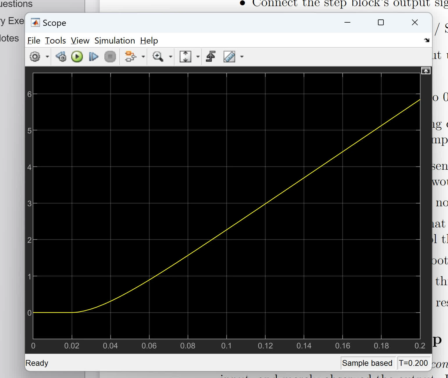
What does the graph represents? What does the first derivative of the graph represent and look like?
Angular position of the motor. The first derivate would be the angular velocity, or the rate of change. It would start at zero (as the first part is flatten) then will keep increasing since the slope is positive.
What is represented by non-linear section?
Represent the system is accelerating
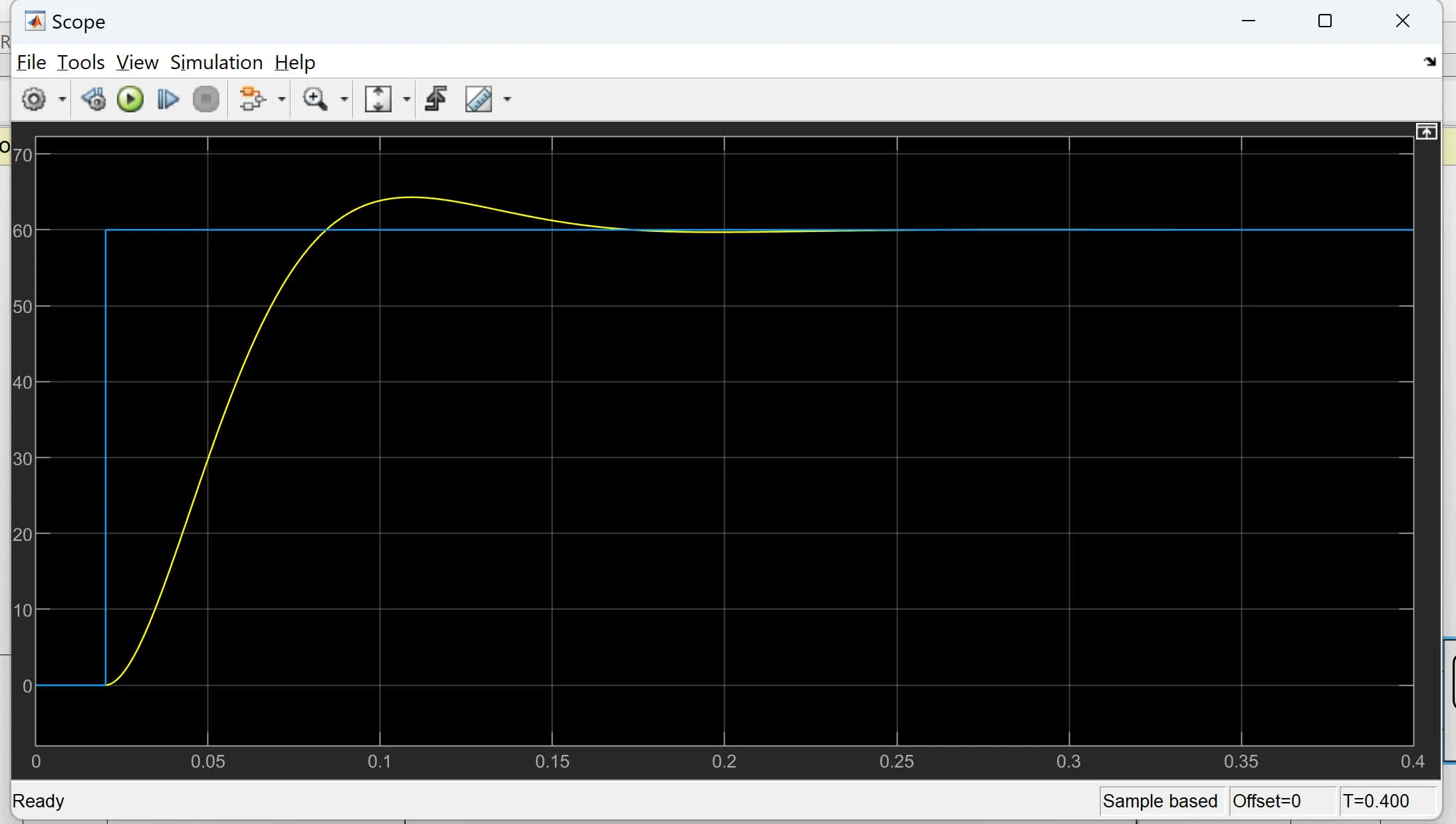
Steady-state error
percent overshoot
settling time of this response
is the response stable with respect to angular position?
5.2 
