Least Squared Regression

question 1.

problem 1.

part 1

Divide the dataset into three parts: 1800 samples for training, 200 samples for validation, and 200 samples for testing. Perform linear OLS (without regularization) on the training samples twice—first with a homogeneous model (i.e., where the y-intercepts are zero) and then with a non-homogeneous model (allowing for a non-zero y-intercept). Report the MSE on both the training data and the validation data for each model

Compare the results. Which approach performs better? Why? Apply the better-performing approach to the test set and report the MSE.

Do you observe significant overfitting in any of the cases?

For homogeneous model, the MSE on training data is 26.1649 and on validation data is 77.0800

Whereas with non-homogeneous model, the MSE on training data is 2.5900 and on validation data is 8.8059
We can observe that non-homogeneous model clearly performs better than the homogeneous models, given a significantly lower MSE (indicates that predictions are closer to the actual value). We can also see the difference between training and validation sets for non-homogeneous models shows better consistency, or better generalisation.

Test set MSE for non-homogeneous model is 2.5900
We observe in both cases that the training MSE is significantly lower than the validation MSE, indicating overfitting. The non-homogeneous model shows a lower difference between training and validation MSE, which suggest there were some overfitting. The homogeneous models show more severe overfitting due to its constraints (forcing intercept to zero).

part 2

Divide the dataset into three parts: 200 samples for training, 1800 samples for validation, and 200 samples for testing. Perform linear OLS (without regularization) on the training samples twice—first with a homogeneous model (i.e., where the y-intercepts are zero) and then with a non-homogeneous model (allowing for a non-zero y-intercept). Report the MSE on both the training data and the validation data for each model

Compare these results with those from the previous part. Do you observe less overfitting or more overfitting? How did you arrive at this conclusion?

For homogeneous model, the MSE on training data is 0.000 and on validation data is 151.2655

Whereas with non-homogeneous model, the MSE on training data is 0.000 and on validation data is 15.8158
We observe an increased in overfitting, given the perfit fit in training data versus validation MSE for both model. We can still see that non-homogeneous models outperform homogeneous models, but the difference between training and validation MSE is significantly higher than the previous case.

This is largely due to smaller training set (200 training samples versus 1800 training samples), models have less data to train on.

problem 2.

part 1

Divide the Dataset into Three Parts:

Training Data: Select 200 data points.

Validation Data: Assign 1800 data points.

Testing Data: Set aside the remaining 200 data points for testing.

Run Regularized Least Squares (non-homogeneous) using 200 training data points. Choose various values of lambda within the range {exp(-2), exp(-1.5), exp(-1), …, exp(3.5), exp(4)}. This corresponds to $\lambda$ values ranging from exp(-2) to exp(4) with a step size of 0.5. For each value of $\lambda$ , Run Regularized Least Squares (non-homogeneous) using 200 training data points. Compute the Training MSE and Validation MSE.

Plot the Training MSE and Validation MSE as functions of lambda.

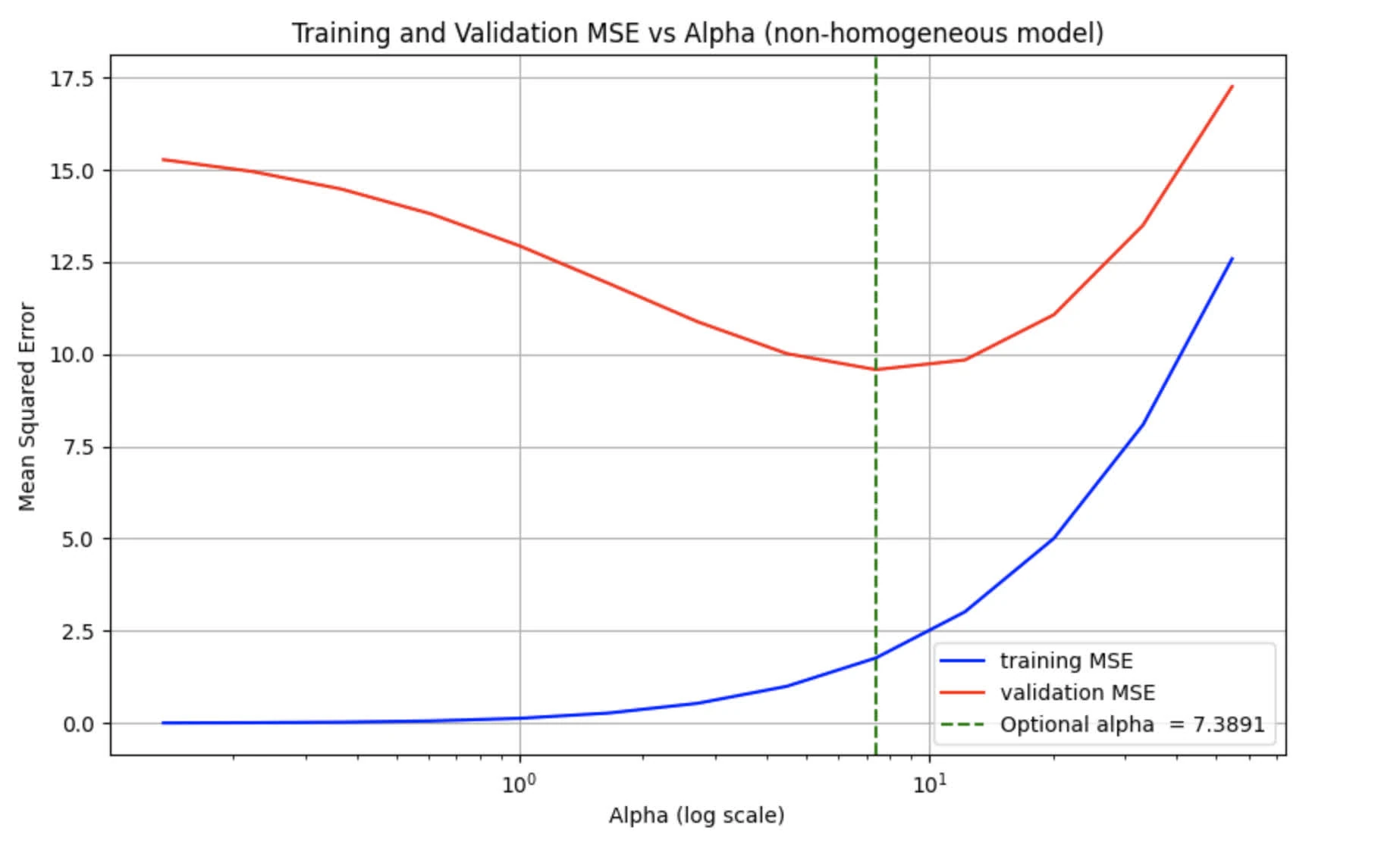
The following is the graph for Training and Validation MSE as functions of lambda.

part 2

What is the best value for lambda? Why?

Use the best value of lambda to report the results on the test set.

Best $\lambda$ would be the one corresponding to lowest point on the validation MSE curve, as it is the one that minimizes the validation MSE. From the graph, we observe it is around $\lambda \approx 7.3891$
Using $\lambda \approx 7.3891$ , we get the following Test MSE around 1.3947

problem 3.

part 1

Choose a preprocessing approach (i.e., select a mapping) that transforms the 900-dimensional data points (900 pixels) into a new space. This new space can be either lower-dimensional or higher-dimensional. Clearly explain your preprocessing approach.

We will use 2D Discrete Cosine Transform (DCT) to transform our data, followed by feature selection to reduce dimensionality by selecting a top-k coefficient.

Reason:

DCT is mostly used in image compression (think of JPEG). Transform image from spatial to frequency domain.
Reduce dimensionality to help with overfitting, given we will only use 200 samples for training.

In this case, we will choose n_coeffs=100

part 2

implement your preprocessing approach.

See the jupyter notebook for more information

part 3

Report the MSE on the training and validation sets for different values of lambda and plot it. As mentioned, it should perform better for getting points. choose the best value of lambda, apply your preprocessing approach to the test set, and then report the MSE after running RLS.

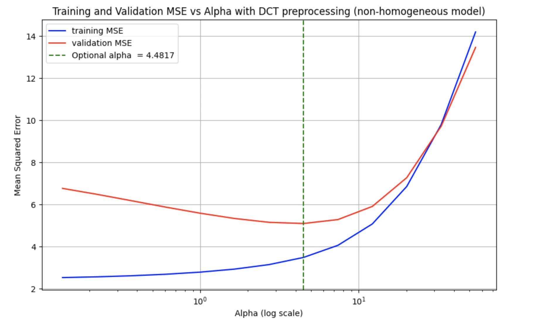
The following graph shows the Training and Validation MSE as functions of $\lambda$ . The optimal alpha is found to be $\lambda \approx 4.4817$

The given Test MSE is found to be around 3.2911

question 2.

problem statement

In this question, we will use least squares to find the best line ( $\hat{y}=ax + b$ ) that fits a non-linear function, namedly $f(x) = 2x - x^3 -1$

For this, assume that you are given a set of $n$ training point $\{ (x^i, y^i)\}^{n}_{i=1} = \{(({i}/{n}), 2({i}/{n})- ({i}/{n})^3- 1)\}^{n}_{i=1}$ .

Find a line (i.e $a,b \in \mathbb{R}$ ) that fits the training data the best when $n \to \infty$ . Write down your calculations as well as the final values for $a$ and $b$ .

Additional notes: $n \to \infty$ assumption basically means that we are dealing with an integral rather than a finite summation. You can also assume $x$ is uniformly distributed on [0, 1]

We need to minimize sum of squared errors:

MSE(a,b) = \int_{0}^{1}(ax^i + b - y^i)^2 dx

We can compute $\mu_{x}, \mu_{y}$ :

\begin{aligned} \mu_{x} &= \int_{0}^{1}x dx = \frac{1}{2} \\ \mu_{y} &= \int_{0}^{1}f(x) dx = \int_{0}^{1}(2x - x^3 - 1) dx = [x^2]^{1}_{0} - [\frac{x^4}{4}]^{1}_{0} - [x]^{1}_{0} = - \frac{1}{4} \end{aligned}

\begin{aligned} \text{Var}(x) &= E[x^2] - (E[x])^2 = \int_{0}^{1}x^2 dx - (\frac{1}{2})^2 = \frac{1}{3} - \frac{1}{4} = \frac{1}{12} \\ \text{Cov}(x,y) &= E[xy] - E[x]E[y] = \int_{0}^{1}x(2x - x^3 - 1) dx - (\frac{1}{2})(-\frac{1}{4}) \end{aligned}

Compute $E[xy] = \int_{0}^{1}(2x-x^4-x)dx = \frac{2}{3} - \frac{1}{5} - \frac{1}{2} = - \frac{1}{30}$ :

Therefore we can compute covariance:

\text{Cov}(x,y) = - \frac{1}{30} + \frac{1}{8} = \frac{11}{120}

Slope $a$ and intercept $b$ can the be computed as:

\begin{aligned} a &= \frac{\text{Cov}(x,y)}{\text{Var}(x)} = \frac{11}{120} \times 12 = 1.1 \\ b &= \mu_{y} - a\mu_{x} = - \frac{1}{4} - \frac{11}{10} \times \frac{1}{2} = - \frac{4}{5} = -0.8 \end{aligned}

Thus, the best-fitting line is $\hat{y} = ax + b = \frac{11}{10}x - \frac{4}{5}$

question 3.

problem statement

In this question, we would like to fit a line with zero y-intercept ( $\hat{y} = ax$ ) to the curve $y=x^2$ . However, instead of minimising the sume of squares of errors, we want to minimise the folowing objective function:
$\sum_{i} [\log {\frac{\hat{y}^i}{y^i}}]^2$
Assume that the distribution of $x$ is uniform on [2, 4]. What is the optimal value for $a$ ? Show your work.

asumption: log base 10

We need to minimize the objective function

\text{Objective}(a) = \text{argmin} \sum_{i} [\log {\frac{\hat{y}^i}{y^i}}]^2

where $\hat{y}^i = ax^i$ and $y^i=(x^i)^2$

Given $x$ is uniformly distributed on [2, 4], we can express the sum as integral:

\begin{aligned} \text{Objective}(a) &= \int_{2}^{4} [\log {\frac{ax}{x^2}}]^2 dx \\ &= \int_{2}^{4} [\log(a) + \log(x) - 2 \log(x)]^2 dx \\ &= \int_{2}^{4} [\log(a) - \log(x)]^2 dx \end{aligned}

let $\ell = \log(a)$ , we can rewrite the objective function as:

\begin{aligned} \text{Objective}(\ell) &= \int_{2}^{4} [\ell - \log(x)]^2 dx \\ &= \int_{2}^{4} [\ell^2 - 2\ell \log(x) + \log^2(x)] dx \\ &= \ell^2 \int_{2}^{4} dx - 2\ell \int_{2}^{4} \log(x) dx + \int_{2}^{4} \log^2(x) dx \end{aligned}

Compute each integral:

\begin{aligned} I_0 &= \int_{2}^{4} dx = 4 - 2 = 2 \\ I_1 &= \int_{2}^{4} \log(x) dx = [x \log(x) - x]^{4}_{2} = 4 \log(4) - 4 - 2 \log(2) + 2 = 4 \log(2) = 6 \log(2) - 2 \\ I_2 &= \int_{2}^{4} \log^2(x) dx \end{aligned}

Given we only interested in finding optimal $a$ , we find the partial derivatives of given objective function:

\frac{\partial}{\partial \ell} \text{Objective}(\ell) = \frac{\partial}{\partial \ell} (\ell^2 I_0 - 2 \ell I_1 + I_2) = 2\ell I_0 - 2I_1

Set to zero to find minimum $\ell$ : $\log(a) = \ell = \frac{I_1}{I_0} = \frac{6 \log(2) - 2}{2} = 3\log(2) - 1$

Therefore, $a_{\text{opt}} = e^{\ell} = e^{3 \log(2) - 1} = e^{3 \log(2)} \times \frac{1}{e} = \frac{8}{e}$

Thus, optimal value for a s $a=8/e$

Least Squared Regression

Étiquette

publié à

modifié à

durée

source

question 1.

problem 1.

problem 2.

problem 3.

question 2.

question 3.

Vous pourriez aimer ce qui suit