PCA and Kernels, from scratch

See also jupyter notebook, pdf, solutions

question 1.

task 1: eigenfaces

implementation of centeralize_data() and pca_components()

def centeralize_data(data):
  return data - (data_mean := np.mean(data, axis=0).reshape(1, -1)), data_mean
 
 
# fmt: off
def pca_components(Vt, n_components): return Vt[:n_components]
# fmt: on

Yields the following when running plot_class_representatives: result

task 2: PCA transformation and reconstructing

part A

Implement pca_tranform

def pca_transform(X, n_components):
  U, s, *result = normalized_svd(X)
  return U[:, :n_components] * s[:n_components], *result

part B

Implement pca_inverse_transform

def pca_inverse_transform(transformed_data, Vt, n_components, data_mean):
  return transformed_data @ pca_components(Vt, n_components) + data_mean

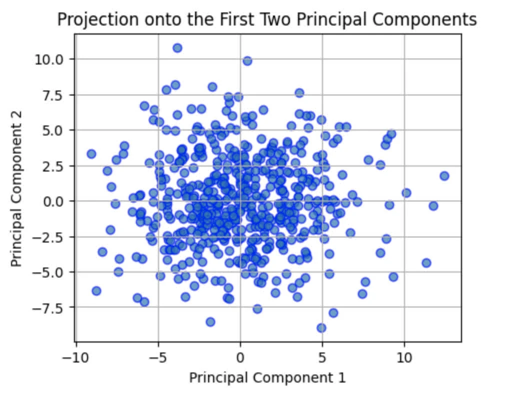
Which yields the following for TNC visualisation:

and LFW visualisation:

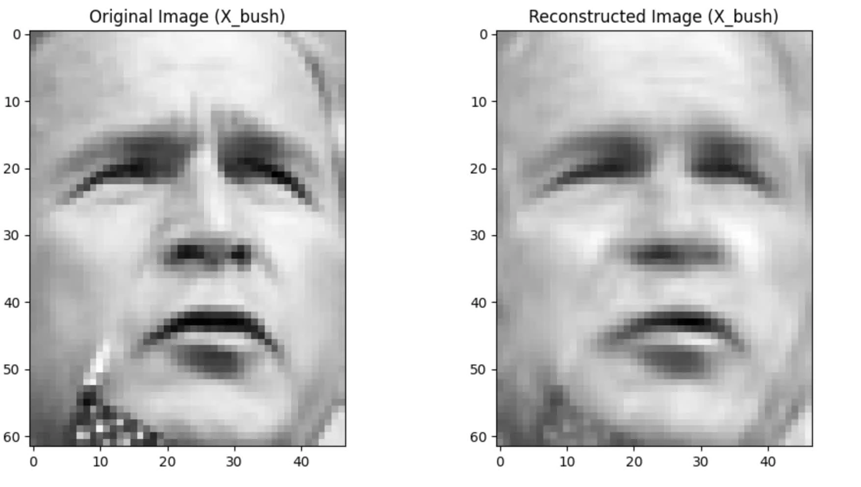
We also expect some loss in information while reconstructing:

task 3: average reconstruction error for LFW

$$\text{error}=\frac{1}{n}\sum_{i=1}^n||x_i-\text{reconstruct}(pca(x_i))||^2_2$$

part A

plot average reconstruction error on training and testing data points

Training code:

# Define the number of components to test in PCA
c_components = [2, 10, 30, 60, 100]
 
# Initialize lists to store the reconstruction errors for training and testing data
train_errors, test_errors = [], []
 
# Initialize deterministic seed
SEED = 42
 
X_train, X_test = train_test_split(X_bush, train_size=400, random_state=SEED)
 
 
# \text{error}=\frac{1}{n}\sum_{i=1}^n||x_i-\text{reconstruct}(pca(x_i))||^2_2
def mse(train_data, reconstructed):
  return np.mean(np.sum((train_data - reconstructed) ** 2, axis=1))
 
 
# Loop through each specified number of components for PCA
for n_components in c_components:
  # Apply PCA and then inverse PCA to the training data
  transformed_train, Vt_train, mean_train = pca_transform(X_train, n_components)
 
  # Calculate the Mean Squared Error (MSE) as the reconstruction error for the training set
  train_errors.append(mse(X_train, pca_inverse_transform(transformed_train, Vt_train, n_components, mean_train)))
  # Normalize the test data. Transform the test data using the train data's PCA components # and reconstruct the test data.
  # Calculate the Mean Squared Error (MSE) as the reconstruction error for the test set
  test_errors.append(mse(X_test,
                         pca_inverse_transform((X_test - mean_train) @ pca_components(Vt_train, n_components).T,
                                               Vt_train, n_components, mean_train)))  # fmt: skip
 
# Print the average reconstruction errors for each number of components
for i, n_components in enumerate(c_components):
  print(f'Components: {n_components}\n\tTrain Error: {train_errors[i]:.4f}\n\tTest Error: {test_errors[i]:.4f}')

yields the following observation

Components: 2
	Train Error: 40.2048
	Test Error: 44.1277
Components: 10
	Train Error: 21.6275
	Test Error: 25.1425
Components: 30
	Train Error: 11.6392
	Test Error: 15.6092
Components: 60
	Train Error: 6.6892
	Test Error: 11.4092
Components: 100
	Train Error: 3.7635
	Test Error: 8.7075

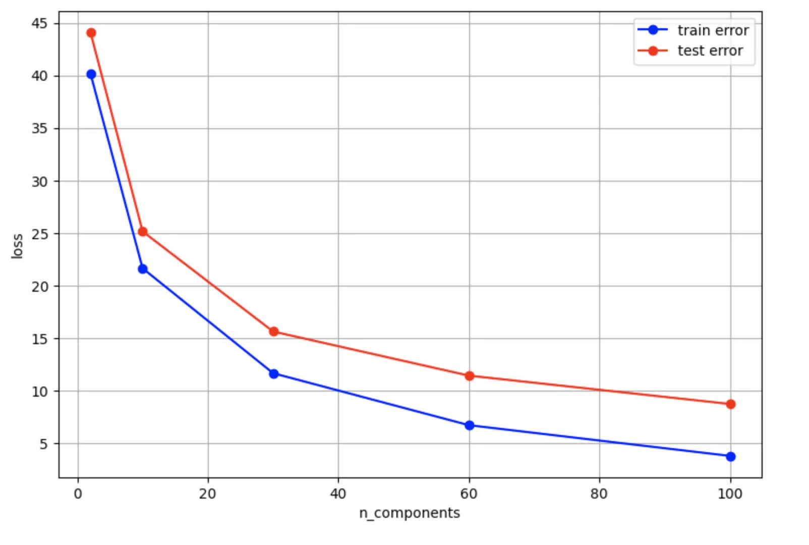
The eval results graph:

part B

1. Explains the difference between the two graphs
2. What would the error be if we compute it for the TNC dataset while using two components and 2000 samples?

1. The following observation can be made:

• Both decreases as the number of components increases (lower means better reconstruction quality). However, we observe test error line (red) is higher than train error (blue). This shows some overfitting given smaller training data size (400) against LFW dataset (which includes 1288 entries)
• Both show diminishing returns, yet this effect is more pronounced on test error
• As n_components increases, we see a decreases in bias (improving reconstruction for both train and test data). However, test error decreases more slowly given later components are less effective in reconstructing features for unseen data

2. Error for average reconstruction error for TNC is shown below:

task 4: Kernel PCA

part A

Apply Kernel PCA and plot transformed Data

Applied a StandardScaler to X_TNC and plot 3x4 grid with the (1,1) being the original data plot, followed by 11 slots for gamma from $[ 0.0001 \cdots 1 ]$. Run on n_components=2

gamma_values = [0.0001, 0.0005, 0.001, 0.005, 0.01, 0.02, 0.05, 0.1, 0.2, 0.5, 1]
n_components = 2
 
# Standardize the features
scaler = StandardScaler()
X_TNC_scaled = scaler.fit_transform(X_TNC)
 
# Create subplots to visualize the transformed data for each gamma
plt.figure(figsize=(20, 15))
 
# Plot the original data before applying Kernel PCA
plt.subplot(3, 4, 1)
plt.scatter(X_TNC_scaled[:, 0], X_TNC_scaled[:, 1], c=Y_TNC, cmap='bwr')
plt.title('Original Data')
plt.xlabel('coord_x')
plt.ylabel('coord_y')
 
# Set the limits for the x and y axes
x_limits = (-4, 4)
y_limits = (-4, 4)
 
# Apply Kernel PCA for each gamma value
for idx, gamma in enumerate(gamma_values):
  # Apply Kernel PCA
  kpca = KernelPCA(n_components=n_components, kernel='rbf', gamma=gamma)
  X_kpca = kpca.fit_transform(X_TNC_scaled)
 
  # Plot the transformed data
  plt.subplot(3, 4, idx + 2)
  plt.scatter(X_kpca[:, 0], X_kpca[:, 1], c=Y_TNC, cmap='bwr')
  plt.title(f'Gamma = {gamma}')
  plt.xlabel('First principal component')
  plt.ylabel('Second principal component')
 
  # Set fixed x and y axis limits
  plt.xlim(x_limits)
  plt.ylim(y_limits)
 
plt.tight_layout()
plt.show()

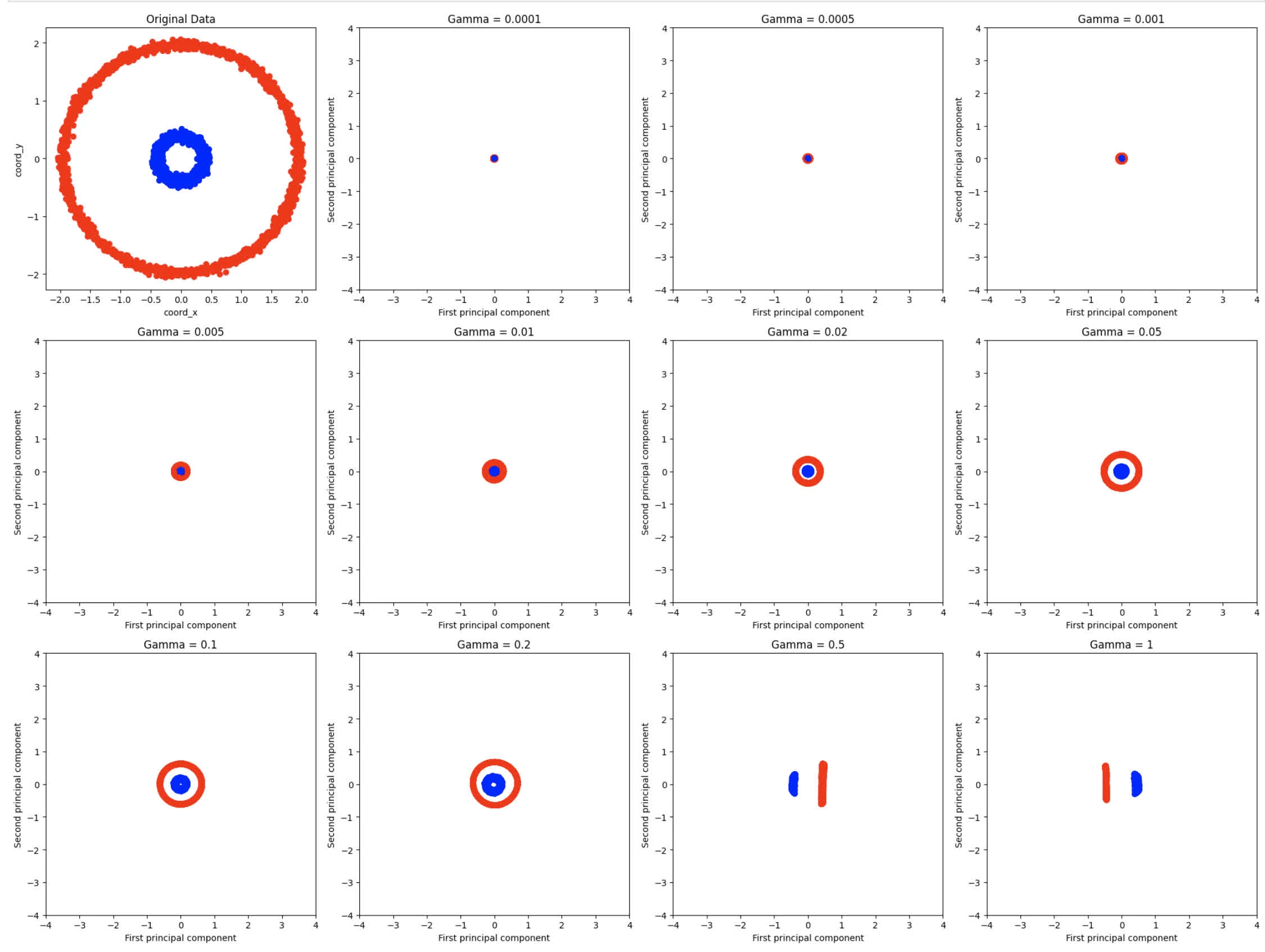
Yield the following graph:

part B

Based on your observations, how does Kernel PCA compare to Linear PCA on this dataset with red and blue labels? In what ways does Kernel PCA affect the distribution of the data points, particularly in terms of how well the red and blue points are organized? Choose the best value(s) for gamma and report it (them). What criteria did you use to determine the optimal gamma value?

Comparison:

• Kernel PCA is more effective in capturing the non-linear relationships in the data, in which we see the spread between blue and red circles, which modify the data distribution. Whereas with linear PCA, it maintains the circular structure, meaning linear PCA doesn’t alter data distribution that much

Effects:

• For small value of gamma $[ 0.0001, 0.0005, 0.001 ]$ the points are highly concentrated, meaning kernels is too wide (this makes sense given that gamma is the inverse of standard deviations)
• For gamma $[ 0.005, \cdots 0.05 ]$, we notice a separation between blue and red circles.
• For gamma $[0.1, 0.2]$ , we start to see similar features from original data entries, albeit scaled down given RBF kernels.
• At gamma $[0.5, 1]$, we notice datasets to spread out, forming elongated features.

For gamma $[ 0.1, 0.2 ]$ seems to provide best representation of the original data

Criteria:

• class separation: how well the blue and red circles are separated from each other
• compact: how tightly clustered the points within each classes are.
• structure preservation: how well the circular nature of the original datasets are preserved.
• dimensionality reduction: how well the data is projected in lower dimensions space

part C

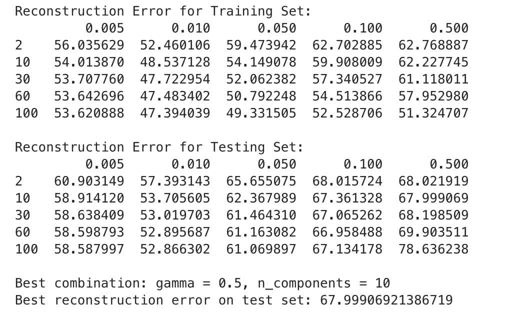
Find best values for reconstruction error of kernel PCA

training loop yields the following:

part D

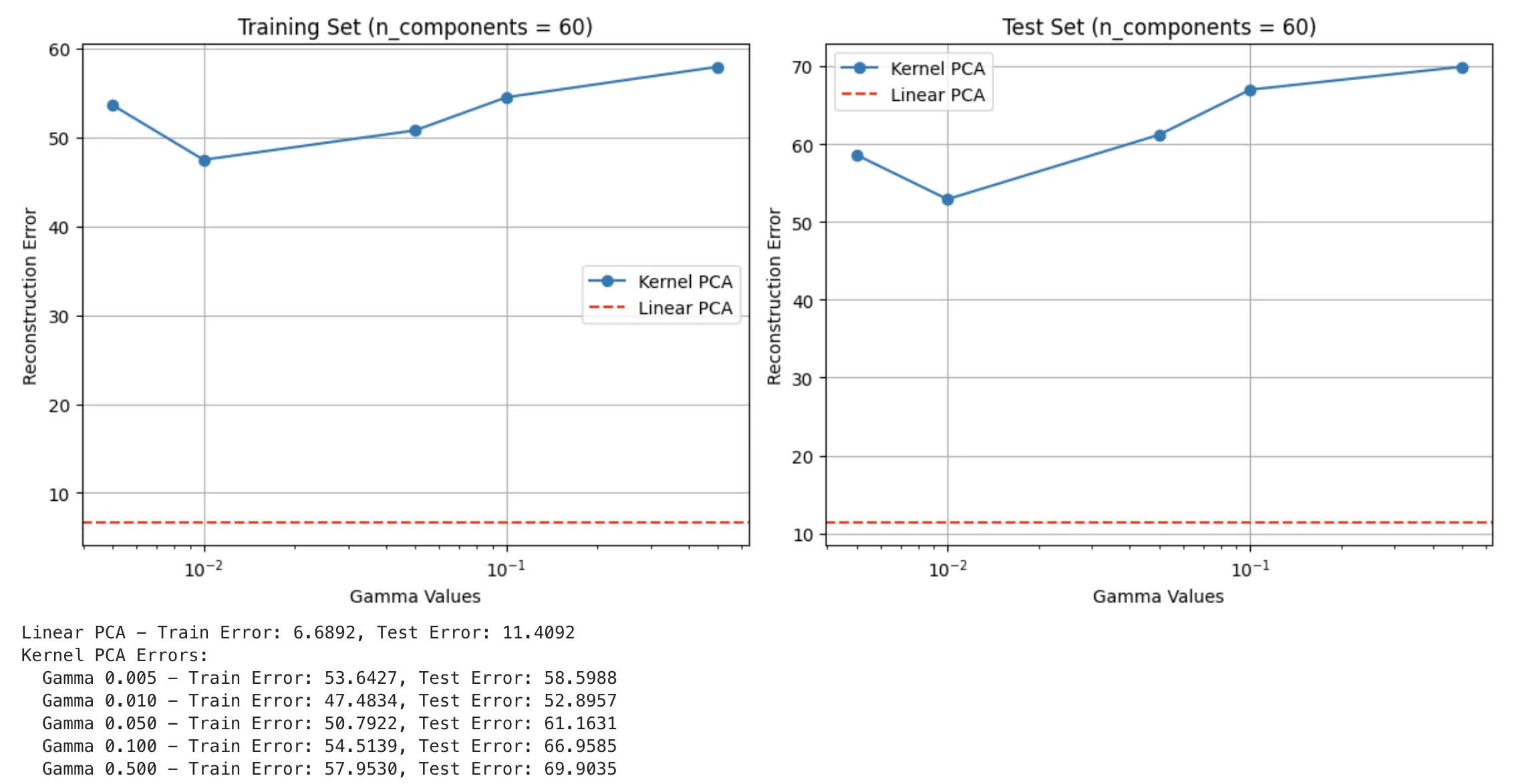
1. Visualisation of Reconstruction Error
2. How does kernel PCA compare to Linear PCA on this dataset? If Kernel PCA shows improved performance, please justify your answer. If Linear PCA performs better, explain the reasons for its effectiveness.

Reconstruction Error from kernel PCA as well as linear PCA:

Performance:

• Linear PCA has significantly better reconstruction error than kernel PCA (6.68 of linear PCA against 47.48 at $\text{gamma}=0.01$ of kernel PCA)
• Regardless of gamma, Kernel PCA shows a lot higher error

Reasoning for Linear PCA:

1. Data characteristic: most likely LFW contains mostly linear relationship between features (face images have strong linear correlations in pixel intensities and structures)
2. Dimensionality: This aligns with Task 3 Part B where we observe same value with n_components=60 for linear PCA
3. Overfitting: less prone to overfitting, given that Kernel PCA might find local optima that overfit given patterns of data (in this case face features). Additionally, RBF is more sensitive to outliers

Explanation why Kernel PCA doesn’t work as well:

1. Kernel: RBF assumes local, non-linear relationships. This might not work with facial data given strong linear correlation among facial features.
2. Gamma: We notice that with $\text{gamma}=0.01$ achieve lowest error, still underperformed comparing to linear PCA.
3. Noise: non-linear kernel mapping are more prone to capture noise or irrelevant patterns in facial images.

---

question 2.

problem statement

“Driving high” s prohibited in the city, and the police have started using a tester that shows whether a driver is high on cannabis. The tester is a binary classifier (1 for positive result, and 0 for negative result) which is not accurate all the time:

• if the driver is truly high, then the test will be positive with probability $1 - \beta_1$ and negative with probability $\beta_1$ (so the probability of wrong result is $\beta_1$ in this case)
• if the driver is not high, then the test will be positive with probability $\beta_2$ and negative with probability $1-\beta_2$ (so the probability of wrong result is $\beta_2$ in this case)

Assume the probability of (a randomly selected driver from the population) being “truly high” is $\alpha$

part 1

What is the probability that the tester shows a positive result for a (randomly selected) driver? (write your answer in terms of $\alpha, \beta_1, \beta_2$)

Probability of a driver being truly high: $P(\text{High}) = \alpha$

Probability of a driver not being high: $P(\text{Not High}) = 1- \alpha$

Probability of a positive test given the dirver is high: $P(\text{Positive} | \text{High}) = 1 - \beta_1$

Probability of a positive test given the dirver is not high: $P(\text{Positive} | \text{Not High}) = \beta_2$

using law of total probability to find overall probability of a positive test result:

$$\begin{aligned} P(\text{Positive}) &= P(\text{Positive} | \text{High}) \cdot P(\text{High}) + P(\text{Positive} | \text{Not High}) P(\text{Not High}) \\ &= (1 - \beta_1) \cdot \alpha + (\beta_2) \cdot (1 - \alpha) \end{aligned}$$

part 2

The police have collected test results for n randomly selected drivers (i.i.d. samples). What is the likelihood that there are exactly $n_{+}$ positive samples among the $n$ samples? Write your solution in terms of $\alpha, \beta_1, \beta_2, n_{+}, n$

Let probability of positive test result for a randomly selected driver is

$$p = P(\text{Positive}) = (1 - \beta_1) \cdot \alpha + (\beta_2) \cdot (1 - \alpha)$$

Now, apply binomial probability to find the likelihood of $n_{+}$ positive samples among $n$ samples:

$$\begin{aligned} P(X=n_{+}) &= \binom{n}{n_{+}} \cdot p^{n_{+}} \cdot (1-p)^{n-n_{+}} \\ &= \binom{n}{n_{+}} \cdot [(1 - \beta_1) \cdot \alpha + (\beta_2) \cdot (1 - \alpha)]^{n_{+}} \\ &\quad \quad \quad \quad \cdot (1 - ((1 - \beta_1) \cdot \alpha + (\beta_2) \cdot (1 - \alpha)))^{n-n_{+}} \\ &= \binom{n}{n_{+}} \cdot [(1 - \beta_1 - \beta_2) \cdot \alpha + \beta_2]^{n_{+}} \cdot (1 - \beta_2 + \alpha \cdot (\beta_1 + \beta_2 - 1))^{n-n_{+}} \\ \end{aligned}$$

part 3

What is the maximum likelihood estimate of $\alpha$ given a set of $n$ random samples from which $n_{+}$ are positive results? In this part, you can assume that $\beta_1$ and $\beta_2$ are fixed and given. Simplify your final result in terms of $n, n_{+}, \beta_1, \beta_2$

Assumption: using nature log ln

MLE of $\alpha$

Let likelikhood function $L(\alpha)$:

$$\begin{aligned} L(\alpha) &= \binom{n}{n_{+}} \cdot p(\alpha)^{n_{+}} \cdot (1-p(\alpha))^{n-n_{+}} \\ \\ \because &\quad p(\alpha) = (1 - \beta_1) \cdot \alpha + \beta_2 \cdot (1-\alpha) \end{aligned}$$

Take log of both sides and drop constant term:

$$\ln L(\alpha ) = n_{+} \ln [p(\alpha)] + (n-n_{+}) \ln [1-p(\alpha)]$$

To find the maximum likelihood, we differentiate with respect to $\alpha$ and set to zero:

$$\begin{aligned} n_{+} \cdot \frac{p^{'}(\alpha)}{p(\alpha )} &- (n-n_{+}) \cdot \frac{p^{'}(\alpha)}{1-p(\alpha )} = 0 \\ \\ \because &\quad p'(\alpha ) = 1 - \beta_1 - \beta_2 \\ \\ \\ \\ n_{+} \cdot \frac{1 - \beta_1 - \beta_2}{p(\alpha )} &= (n-n_{+}) \cdot \frac{1 - \beta_1 - \beta_2}{1-p(\alpha )} \\ \\ n_{+} - n_{+} p(\alpha ) &= n p(\alpha) - n_{+} p(\alpha) n_{+} = np(\alpha) \end{aligned}$$

Substituting $p(\alpha) = (1 - \beta_1) \cdot \alpha + \beta_2 \cdot (1-\alpha)$:

$$\begin{aligned} n_{+} &= n [(1-\beta_1) \cdot \alpha + \beta_2 \cdot (1-\alpha)] \\ \frac{n_{+}}{n} &= (1-\beta_1-\beta_2) \cdot \alpha + \beta_2 \\ \\ \\ \\ \text{MLE for } \hat{\alpha} &= \frac{\frac{n_{+}}{n} - \beta_2}{1 - \beta_{1} - \beta_{2}} \\ &= \frac{n_{+} - n \cdot \beta_{2}}{n - n\cdot \beta_{1} - n\cdot \beta_{2}} \end{aligned}$$

part 4

What will be the maximum likelikhood estimate of $\alpha$ for the special cases of

• $(i) \beta_{1} = \beta_{2} = 0$
• $(i) \beta_{1} = \beta_{2} = 0.5$
• $(i) \beta_{1} = 0.2, \beta_{2} = 0.3$

For $(i) \beta_{1} = \beta_{2} = 0$: $\hat{\alpha} = \frac{n_{+}}{n}$

For $(i) \beta_{1} = \beta_{2} = 0.5$: $\hat{\alpha} = \text{undefined}$

note: this makes sense, given when the test is completely random, then there is no information about true proportion of high drivers.

For $(i) \beta_{1} = 0.2, \beta_{2} = 0.3$: $\hat{\alpha} = \frac{n_+ - 0.3n}{0.5n} = \frac{2n_{+}}{n} - \frac{3}{5} = \frac{2n_+}{n} - 0.6$