Economics for engineer, a guide.

samples.

4.b 11.e 12.c 13.d 14.b 15.a 16.e 17.c 18.c 19.b 20.c 21.b 22.c 23.b 24.a 25.a 26.e 27.a 28.e 29.a 30.a

---

net value function

$$\text{NVF}=\text{benefit}-\text{cost}$$

conversion factors

marginal value change.

extra net value obtained for one more item

$$\Delta NV=NV(x+1)-NV(x)$$ Lien vers l'original

optimisation

model-based

• conclusions from the model of the system

Components:

• decision variables
• constraints
• objectives
• functions: mathematical function that determines the objective as a function of decision variable

$$\begin{array}{rlrl}\underset{x}{\min }\varphi =f(x)& & \leftarrow & \text{Objective function}\\ \text{s.t}& & \leftarrow & \text{Constraints}\\ h(x)=0& & \leftarrow & \text{Equality constraints}\\ g(x)\le 0& & \leftarrow & \text{Inequality constraints}\\ x_{lb}\le x\le x_{ub}& & \leftarrow & \text{Bounds}\end{array}$$

decision variables

discrete.

limited to a fixed or countable set of values

$$x_{\mathcal{D}}\mid a\in \mathcal{I}=\{1,2,3,4,5\}$$

continuous.

can take any value within a range

$$x_{\mathcal{C}}\subset \mathcal{R}$$

constraints

• physical limitations: cannot purchase negative raw materials

• model assumptions: assumptions about the system

domain of a definition

a decision upper and lower bounds ($x^{\mathcal{U}}$ and $x^{\mathcal{L}}$)

Properties

• Active/binding: $\exists x^{\ast }\mid g(x^{\ast })=0$

• Inactive: $\exists x^{\ast }\mid g(x^{\ast })<0$

graphing models

feasible set of an optimization model

The collection of decision variables that satisfy all constraints

$$\mathcal{S}\triangleq \{x:g(x)\le 0,h(x)=0,x^L\le x\le x^U\}$$

outcomes

optimal value

the optimal value ${\varphi }^{\ast }$ is the value of the objective at the optimum(s)

$${\varphi }^{\ast }\triangleq \varphi (x^{\ast })$$

Constraints satisfy, but it is not binding

Linear optimization problems

$$\begin{array}{rl}\underset{x_1,x_2}{\min }\varphi & =50x_1+37.5x_2\\ & \text{s.t}\\ 0.3x_1+0.4x_2& \ge 2000\\ 0.4x_1+0.15x_2& \ge 1500\\ 0.2x_1+0.35x_2& \le 1000,\\ x_1& \le 9000\\ x_2& \le 6000\\ x_i& \ge 0\end{array}$$

See also Linear Optimization

Lien vers l'original

Linear optimization:

\begin{align*}
\min_{x} \phi = c^\mathbf{T} \mathcal{x} & &\leftarrow &\space \text{Objective function} \\\
\text{s.t} & &\leftarrow &\space \text{Constraints} \\\
A_h \mathcal{x} = \mathcal{b}_h & &\leftarrow &\space \text{Equality constraints} \\\
A_g \mathcal{x} \leq \mathcal{b}g \leq 0 & &\leftarrow &\space \text{Inequality constraints} \\\
\mathcal{x}_{lb} \leq \mathcal{x} \leq \mathcal{x}_{ub} & &\leftarrow &\space \text{Variable Bounds}
\end{align*}

Lien vers l'original

time value of money

interest

Interest $I$ is the compensation for loaning money.

interest rate

$i=\frac{I}{P}$. Thus $F=P(1+i)$

Simple interests

$I_{\text{each}}=P\times \frac{i}{\text{year}}$, total interest $I=I_{\text{each}}\times N_{\text{year}}$

$F_n=P(1+ni)$

Compound interests

$F_n=P(1+i{)}^n$

nominal interest rates

$r$ is the equivalent yearly rate if interest is withdrawn so it doesn’t compound. (i.e: $r=mi$ where $m$ is the number of compounding periods per year)

effective annual interest rates

$i_{\text{eff}}=(1+\frac{r}{m}{)}^m-1$

effective interest rates

how much interest do you accrue after a year if nominal rate is 12%? $F=P(1+i{)}^m=P(1+\frac{r}{m}{)}^m$

continuous compounding

$F=P{e}^{ry}$

net present value

$$\text{NPV}={\text{CF}}_0+\sum _{n=1}^N\frac{{\text{CF}}_n}{(1+i{)}^n}$$

where ${\text{CF}}_0$ is the initial cash flow, ${\text{CF}}_n$ is the cash flow at the end of the $n^{th}$ period, $i$ is the effective interest rate

discount rate

Present value $PV=\frac{{\text{CF}}_t}{(1+r_d{)}^t}$, where ${\text{CF}}_t$ is cash flow happening in $t$ years in the future, and $r_d$ is the discount rate.

sources: opportunity cost, inflation, risk, time preference, inflation, option premium

regular deposit: Future value $FV=A{\sum }_{k=0}^{n-1}(1+i{)}^k=A\frac{(1+i{)}^n-1}{i}$ where $A$ is the monthly, or time period, deposit.

fraction of last payment that was interest was $\frac{i}{1+i}$, principal of the last payment is $A=F_{\text{last}}(1+i)$

geometric series

$$\sum _{k=0}^{n-1}{r}^k=\frac{1-r^n}{1-r}$$

inflation

real vs. nominal

nominal value refers to actual cash flow at the time it hapens, real value refers to equivalent amount of value at reference time, converted using inflation rates.

real dollar $R=\frac{{\text{CF}}_n}{(1+r_i{)}^n}$, where ${\text{CF}}_n$ is the nominal cash flow at time $n$, and $r_i$ is the effective yearly inflation rate.

internal rate of return

the discount rate that results in a NPV of zero (break-even scenario)

$${\text{CF}}_0+\sum _{n=1}^N\frac{{\text{CF}}_n}{(1+r_{\text{IRR}}{)}^n}=0$$

minimum acceptable rate of return

a rate of return set by stakeholders that must be earned for a project to be accepted

real vs. nominal MARR: real MARR is MARR if returns are calculated using real dollars, whereas nominal MARR is MARR if returns are calculated using nominal dollars.

${\text{MARR}}_{\text{real}}=\frac{1+\text{MARR}}{1+f}-1$ where $f$ is the inflation rate

risk management and stochastic modelling

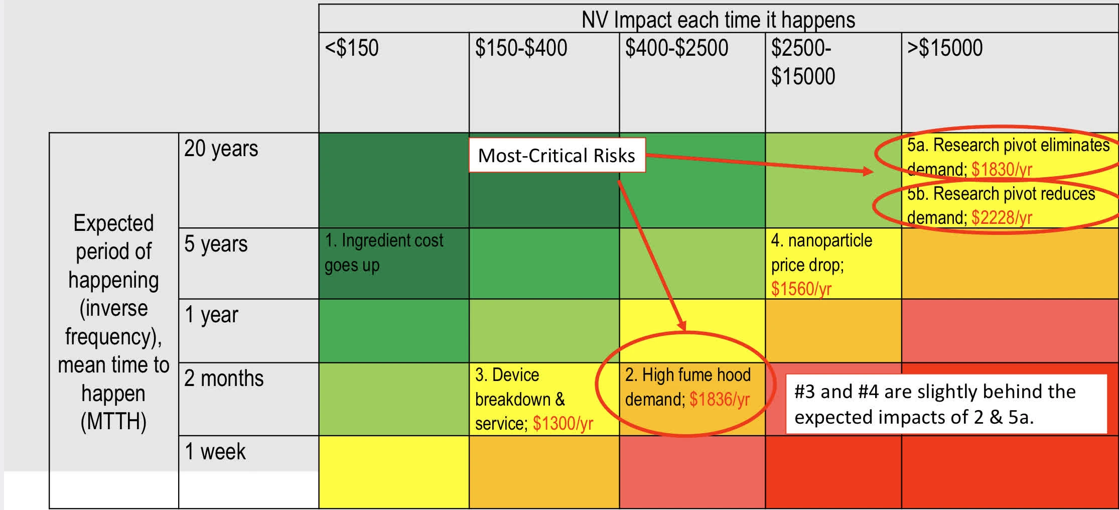
Convert to dollar/wk to base calculation on same unit

uncertainty, evaluating likeliness and potential impact, organize to risk matrix, determine expected impact, then propose mitigation strategies

expected impact

the chance it happens multiplied by the impact it will have if it happens. $\text{E[NPV]}={\sum }_i\text{NPV}(x_i)p(x_i)$

Then use this to create necessary mitigation

NPV with risk and uncertainty

probability distribution

$p(x)$ of a discrete random variable $x$: Normalization requires that ${\sum }_{i}p(x_i)=1$

PDF (probability density function) $f(x)$ of a continuous random variable $x$: Normalization requires that $\int p(x)dx=1$

expected value for calculating stochastic to deterministic

of function $f(x)$ is $\text{E}[f]={\sum }_{i}f(x_i)p(x_i)$ for discrete random variable $x$ with probability distribution $p(x)$

of function $f(x)$ is $\text{E}[f]={\int }_{x}f(x)p(x)dx$ for continuous random variable $x$ with PDF $p(x)$

Normal distribution

$f(x)=\frac{1}{\sigma \sqrt{2\pi }}{e}^{-\frac{(x-\mu {)}^2}{2{\sigma }^2}}$

NORM.DIST(x, mean, stddev, cumulative): cumulative is 1 for CDF, 0 for PDF NORM.INV(RAND(), 0.5, 0.05): draw values from a normal distribution with mean 0.5 and stddev 0.05

non-linear deterministic and stochastic models

mean value ${\mu }_x$ of a random variable $x$ is its own expected value $\text{E}[x]$, variance ${\sigma }_x^2$ is the expected value of the squared deviation from the mean $\text{E}[(x-{\mu }_x{)}^2]$, and stddev ${\sigma }_x$

central limit theorem

sample size becomes large enough, the distribution of the sample mean will be approximately normally distributed, regardless of the distribution of the population, using Monte-Carlo simulation

Expected value of linear and nonlinear functions: suppose $x$ and $y$ are independent random variables with means ${\mu }_x$ and ${\mu }_y$, and variances ${\sigma }_x^2$ and ${\sigma }_y^2$, then $E[x^2]={\sigma }_x^2-{\mu }_x^2$, $E[xy]=\int \int xy{p}_x{p}_{y}dxdy=\int x{p}_{x}dx\int y{p}_{y}dy={\mu }_x{\mu }_y$

Dealing with 12 months per year: saying outcomes over a year should be normally distributed (CLT), with a mean given by expected value of monthly outcome and stddev given stddev of outcome divided by square root of the # of rolls ($\sqrt{12}$)

---

project management and CPM

• scope, cost, time to maximize quality

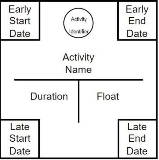
WBS (work breakdown structure): hierarchical decomposition of the total scope of work

CPM (critical path method): determine the longest path through the network, the critical path, and the shortest time to complete the project

crashing a project means using additional resources to shorten a specific task

supply and demand

market equilibrium: where supply and demand curves intersect, quantity demanded equals quantity supplied. shift to right: greater demand, higher price, higher quantity. shift to left: lower demand, lower price, lower quantity. factors of production: land, labour, capital, entrepreneurship determinants of demand:

• price: quantity demanded $Q_d$ falls when price $P$ rises and vice versa
• prices of related goods: substitutes and complements determinants of supply:
• price: quantity supplied $Q_s$ rises when price $P$ rises and vice versa
• factors of productions
• fiscal policies, taxes, regulation

elasticity: how responsive quantity demanded or supplied is to a change in price.

Surplus when $Q_s>Q_d$, shortage when $Q_s<Q_d$.

Elasticity of demand: $E_d=\frac{\%\Delta Q_d}{\%\Delta P}=\frac{\mid \frac{P}{Q_D}\mid }{\mid \frac{dP}{d{Q}_D}\mid }$

Elasticity of supply: $E_s=\frac{\%\Delta Q_s}{\%\Delta P}=\frac{\mid \frac{P}{Q_S}\mid }{\mid \frac{dP}{d{Q}_S}\mid }$

higher slope corresponds to lower elasticity: inelastic, lower slope corresponds to higher elasticity: elastic

Demand elasticity: $E_D<1$ means if price increases by 5% then demand will decrease by less than 5%, inelastic. $E_D>1$ means if price increases by 5% then demand will decrease by more than 5%, elastic.

taxes

arbitrary lower the equilibrium quantity,

price seen by consumers vs. suppliers changes depends on relative elasticities of demand and supply: more price change will end up on consumer side

quantities change depends on total elasticities of demand and supply: more elastic means more quantity change.

subsidies

arbitrary increase the equilibrium quantity,

price seen by consumers vs. suppliers changes depends on relative elasticities of demand and supply: more price change will end up on consumer side

quantities change depends on total elasticities of demand and supply: more elastic means more quantity change.

behavioural economics

invisible hand of the market: self-interest of individuals leads to the best outcome for society as a whole, in a free market economy, as rational actors are motivated by incentives.

perfect competition: wheat (control of price none, low barrier to entry, high # of producers, products are identical) monopolistic competition: restaurants (control of price low, low barrier to entry, high # of producers, products are similar) oligopoly: airlines (control of price high, high barrier to entry, few producers, products are similar) monopoly: utilities (control of price high, high barrier to entry, one producer, unique product)

game theory, most notable The Prisoner’s Dilemma

anti-trust legislation: prevent monopolies, promote competition, protect consumers

behavioural economics: + psychology to look at reasons people make irrational decisions

“bounded rationality”: you don’t have perfect information, and understand there’s an opportunity cost to get it

law of demand and ultimatum game: people will pay less for a good if they can get it elsewhere for less, even if they value it more than the price they pay.

Cooperation: R. Axelrod’s The Evolution of Cooperation propose a “strategy”, what you do dependent on what the other person does.

PPF (production possibility frontier): trade-offs between two goods, given a fixed amount of resources.

risk aversion: people prefer a certain outcome to a risky one, even if the expected value of the risky one is higher. ⇒ assume that the given investment is loss, then calculate based on margin gains

tax, incentives and depreciations

income, corporate, property, sales

personal income tax: progressive tax rate corporate tax: flat tax rate, regardless of income level → net income: subtracting expenses from gross income.

profit on investments will be tax. If yields loss, then offset the loss against the profits from another to pay less tax overall.

optimization strategies: minimize liabilities, timing of expenditures → incorporate into financial models, do sensitivity analysis

before-tax MARR: set MARR high enough to include taxes that need to be paid ⇒ for investment’s gross profit after-tax MARR: if tax is explicitly accounted for in the cash flows of the project, then MARR should be lower ⇒ for final investment decisions

$$MAR{R}_{\text{after-tax}}=MAR{R}_{\text{before-tax}}\times (1-\text{corporate tax rate})$$

incentives: tax credits, tax reliefs, programs to encourage certain activities depreciation: due to use-related physical loss, technological obsolescence, functional loss, market fluctuation.

Deprecation is a non-cash expense, but reduces the taxable income of a business. Can deduct annually by spreading the cost of an asset over its useful life.

affects NPV (net present value), IRR (internal rate of return), and payback period calculation

Market value: actual value of the asset can be sold for, estimated Book value: deprecated value of the asset, using a depreciation model Salvage value: estimated value of the asset at the end of its useful life

value calculations

Depreciation in year $n$ $D(n)$ is the decline in book value over that year: $BV(n)=BV(n-1)-D(n)$

Salvage value $SV$ is the book value at object’s EOL: $SV=BV(N)=MV(0)-{\sum }_{n=1}^{N}D(n)$

Straight-line depreciation

spreads uniformly over useful life, SLD of a period $D_{\text{sl}}(n)=\frac{\text{Purchase price}-\text{Salvage value after N periods}}{\text{N periods of useful life}}$.

book value at end of $n^{th}$ year: $B{V}_{\text{sl}}(n)=P-n\times \frac{P-S}{N}$

Declining-balance depreciation

different assets are classified into classes: $D_{\text{db}}(n)=B{V}_{\text{db}}(n-1)\times d(\text{depreciation rate})$, such that book value at the end of a period $B{V}_{\text{db}}(n)$ is $B{V}_{\text{db}}(n)=P(1-d{)}^n$

given salvage value $S$ and period of useful life $N$, depreciation rate $d=1-\sqrt[N]{\frac{S}{P}}$

Sum-of-years-digits depreciation

$D_{\text{syd}}(n)=\frac{N-n+1}{{\sum }_{i=1}^{N}i}\times (P-S)$

Unit of production depreciation

$D_{\text{uop}}(n)=\frac{\text{units produced of period}}{\text{life in \# of units}}\times (P-S)$

assumes a SLD but vs. # of units rather than time.