Second-order systems

problem 1.

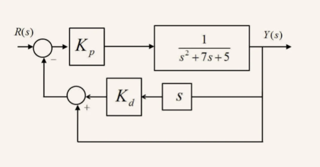
Consider the following system:

Question

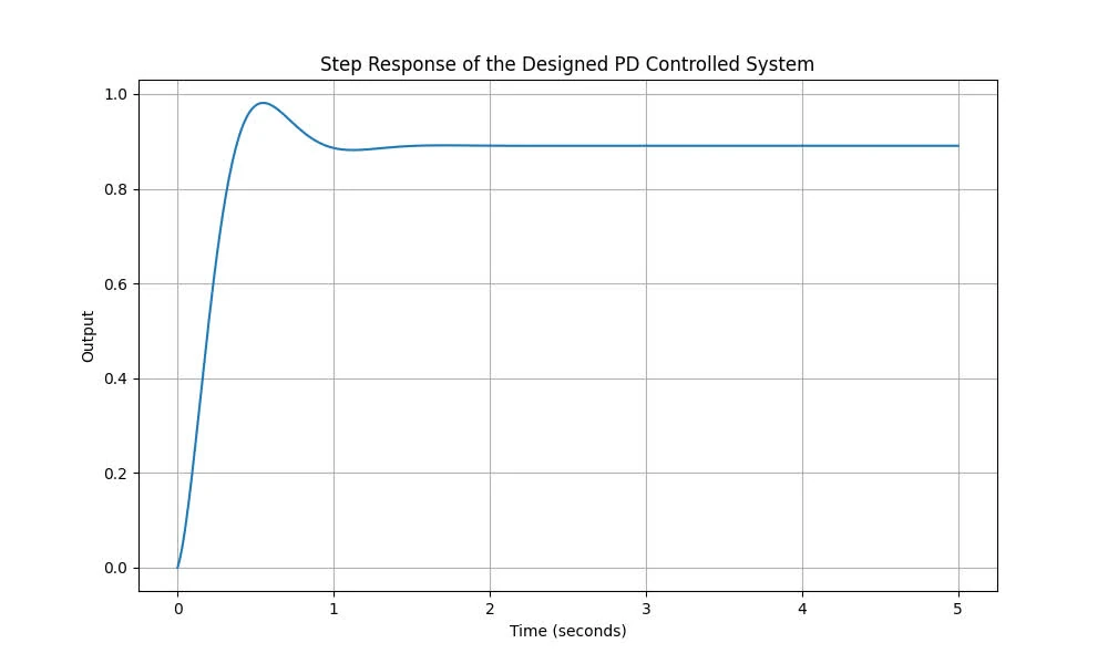
Using the properties of second-order systems, determine $K_p$ and $K_d$ such that the overshoot is 10 percent and the settling time is 1 second. Confirm that your design meets the requirements by plotting the step response.

Given the percent overshoot $\%OS$ and settling time based on the damping ratio $\zeta$ and natural frequency $\omega_n$:

$$\begin{align*} \%{OS} &= e^{\frac{-\zeta\pi}{\sqrt{1-\zeta^2}}} \times 100 \% \\\ T_s &= \frac{4}{\zeta\omega_n} \end{align*}$$

For 10% overshoot, we can solve for $\zeta$: $\zeta = \frac{-\ln(\%{OS}/100)}{\sqrt{\pi^2 + \ln^2(\%{OS}/100)}} \approx 5.916 \times e{-1}$. For 1 second settling time, we can solve for $\omega_n$: $\omega_n = \frac{4}{\zeta T_s} \approx 6.76 \space rad \space s$.

Given second-order systems’ transfer function:

$$G(s) = \frac{\omega_n^2}{s^2 + 2\zeta\omega_n s + \omega_n^2}$$

and the transfer function of the PID controller in the given system is given by:

$$G_c(s) = K_p + K_d s$$

The transfer function is then followed by:

$$T(s) = G(s) G_c(s) = \frac{K_p + K_d s}{s^2 + 7s + 5}$$

We then have $\omega_n$ and $\zeta$ to solve for $K_p$ and $K_d$:

$$\begin{align*} 7+K_pK_d &= 2\zeta\omega_n \\\ 5+K_d &= \omega_n^2 \end{align*}$$

Thus, $K_p = 40.784365358764106$ and $K_d = 0.9999999999999991$.

The following is the code snippet for generating the graphs and results:

p1.py

from scipy.optimize import fsolve
import numpy as np
import matplotlib.pyplot as plt
from scipy.signal import TransferFunction, step
 
OS, Ts = 0.10, 1.0
zeta = fsolve(lambda z: np.exp(-z*np.pi/np.sqrt(1-z**2)) - OS, 0.5)[0]
wn = 4 / (zeta * Ts)
 
# Coefficients from the standard second-order system
a1 = 2 * zeta * wn  # coefficient of s
a0 = wn**2          # constant coefficient
 
# Equating the coefficients to solve for Kp and Kd
# 7 + Kd = a1 and 5 + Kp = a0
Kd = a1 - 7
Kp = a0 - 5
 
# Confirm the design by plotting the step response
# First, define the transfer function of the closed-loop system with the calculated Kp and Kd
G = TransferFunction([Kd, Kp], [1, 7+Kd, 5+Kp])
 
# Now, generate the step response of the system
time = np.linspace(0, 5, 500)
time, response = step(G, T=time)
 
print(Kp, Kd, zeta, wn)
# Plot the step response
plt.figure(figsize=(10, 6))
plt.plot(time, response)
plt.title('Step Response of the Designed PD Controlled System')
plt.xlabel('Time (seconds)')
plt.ylabel('Output')
plt.grid(True)
plt.show()

---

problem 2.

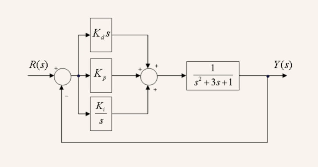
Consider the following system:

set a.

If $K_d=K_p=K_i = 1$, is the system stable? (Please determine this by explicitly finding the poles of the closed-loop system and reasoning about stability based on the pole locations.)

Given that $K_d = K_p = K_i = 1$, The PID controller transfer function is:

$$C(s) = K_p + \frac{K_i}{s} K_d s = 1 + \frac{1}{s} + s$$

The open-loop transfer function is given by: $G(s) = C(s) P(s) = (1 + s + \frac{1}{s}) \frac{1}{s^2 + 3s + 1}$.

Thus the closed-loop transfer function is given by $T(s) = \frac{G(s)}{1 + G(s)} = \frac{s^3 + s^2 + 1}{s^3 + s^2 + 4s + 2}$.

We need to solve $s^3 + s^2 + 4s + 2 = 0$ to find the poles of the closed-loop system.

import numpy as np
print(np.roots([1,1,4,2]))

which yields [-0.23341158+1.92265955j -0.23341158-1.92265955j -0.53317683+0.j] as poles. Since all the poles have negative real parts, the system is stable.

set b.

Fix $K_i = 10$. Using the Routh-Hurwitz criterion, determine the ranges of $K_p$ and $K_d$ that result in a stable system.

The open-loop transfer function is given by

$$G(s) = C(s) P(s) = (K_p + \frac{K_i}{s} + K_d s) \frac{1}{s^2 + 3s + 1} = \frac{K_d s^2+K_p s + 10}{s^3+3s^2+s}$$

The characteristic equation of the closed-loop system is given by $1 + G(s) = 0$:

$$\begin{align*} 1 + \frac{K_d s^2+K_p s + 10}{s^3+3s^2+s} &= 0 \\\ s^3+3s^2+s + K_d s^2 + K_p s + 10 &= 0 \\\ s^3 + (3+K_d) s^2 + (K_p + 1)s + 10 &= 0 \end{align*}$$

Applying the Routh-Hurwitz criterion, we have the following table:

from sympy import symbols, Matrix
Kd, Kp = symbols('Kd Kp')
a0 = 10
a1 = Kp + 1
a2 = 3 + Kd
a3 = 1
 
routh = Matrix([
  [a3, a1],
  [a2, a0],
  [a1 - (a2*a3)/a3, 0],
  [a0, 0]
])
 
print(routh)

which results in the following table:

Matrix([[1, Kp + 1], [Kd + 3, 10], [-Kd + Kp - 2, 0], [10, 0]])

The conditions for stability from the Routh-Hurwitz criterion states that all the elements in the first column of the Routh array must be positive. Thus, we have the following inequalities:

$$\begin{align*} K_d + 3 &> 0 \\\ -K_d + K_p - 2 &> 0 \end{align*}$$

Solving for $K_d$ and $K_p$ yields the following ranges:

$$\begin{align*} K_d &> 0 \\\ K_p &> 2 \end{align*}$$

set c.

For the system in the first question, suppose that you want the steady-state error to be $10\%$. What should the values of $K_p$ and $K_d$ be? (Hint: the system is not in the unity gain form that we discussed in detail in lecture, so be careful.)

The open-loop transfer function is given by:

$$G(s)H(s) = (K_p + K_d s)\frac{1}{s^2+7s+5}$$

The transfer function for closed-loop is given by:

$$T(s) = \frac{G(s)H(s)}{1+G(s)H(s)}$$

From final value theorem, the steady-state error is given by

$$\lim_{s\to0}s\cdot R(s) \cdot (1-T(s))$$

For step input $R(s) =\frac{1}{s}$ we got

$$SSE = 0.1 = \lim_{s\to0} s \cdot \frac{1}{s} \cdot (1 - \frac{K_p + K_d s}{s^2+7s +5 + K_p + K_d s})$$

$K_p = \frac{5}{8}$