Tout ce qu'il faut savoir sur la conception des systèmes de contrôle See also source for code and jupyter notebook
Book: ISBN: 978-1-119-47422-7 and pdf
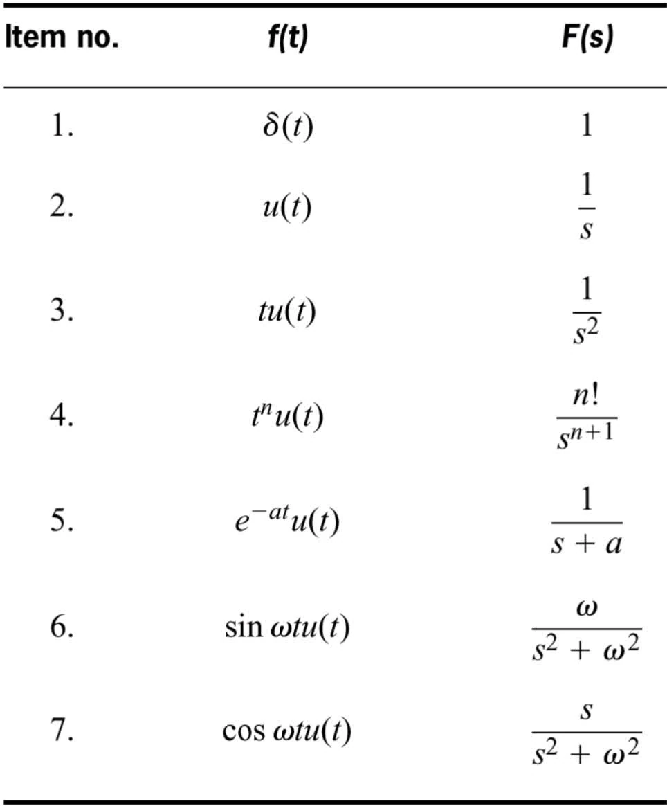
sp.Heaviside(t)
is u ( t ) u(t) u ( t )
import sympy
import sympy as sp
from symbol import symbols , apart , inverse_laplace_transform , simplify
from sympy . abc import s , t
See notes
Transfer function
n t h n^{th} n t h order linear, time-invariant (LTI) differential equation:
a n d n c ( t ) d t n + a n − 1 d n − 1 c ( t ) d t n − 1 + ⋯ + a 0 c ( t ) = b m d m r ( t ) d t m + b m − 1 d m − 1 r ( t ) d t m − 1 + ⋯ + b 0 r ( t ) a_n \frac{d^n c(t)}{dt^n} + a_{n-1} \frac{d^{n-1} c(t)}{dt^{n-1}} + \cdots + a_0 c(t) = b_m \frac{d^m r(t)}{dt^m} + b_{m-1} \frac{d^{m-1} r(t)}{dt^{m-1}} + \cdots + b_0 r(t) a n d t n d n c ( t ) + a n − 1 d t n − 1 d n − 1 c ( t ) + ⋯ + a 0 c ( t ) = b m d t m d m r ( t ) + b m − 1 d t m − 1 d m − 1 r ( t ) + ⋯ + b 0 r ( t )
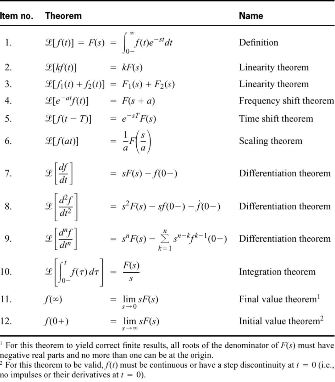
takes Laplace transform from both side
a n s n C ( s ) + a n − 1 s n − 1 C ( s ) + ⋯ + a 0 C ( s ) and init terms for c ( t ) = b m s m R ( s ) + b m − 1 s m − 1 R ( s ) + ⋯ + b 0 R ( s ) and init terms for r ( t ) \begin{aligned}
& a_n s^n C(s) + a_{n-1} s^{n-1} C(s) + \cdots + a_0 C(s) \text{ and init terms for } c(t) \\
& = b_m s^m R(s) + b_{m-1} s^{m-1} R(s) + \cdots + b_0 R(s) \text{ and init terms for } r(t) \\
\end{aligned} a n s n C ( s ) + a n − 1 s n − 1 C ( s ) + ⋯ + a 0 C ( s ) and init terms for c ( t ) = b m s m R ( s ) + b m − 1 s m − 1 R ( s ) + ⋯ + b 0 R ( s ) and init terms for r ( t )
assume initial conditions are zero
( a n s n + a n − 1 s n − 1 + ⋯ + a 0 ) C ( s ) = ( b m s m + b m − 1 s m − 1 + ⋯ + b 0 ) R ( s ) C ( s ) R ( s ) = G ( s ) = b m s m + b m − 1 s m − 1 + ⋯ + b 0 a n s n + a n − 1 s n − 1 + ⋯ + a 0 \begin{aligned}
(a_n s^n + a_{n-1} s^{n-1} + \cdots + a_0)C(s) &= (b_m s^m + b_{m-1} s^{m-1} + \cdots + b_0)R(s) \\[8pt]
\frac{C(s)}{R(s)} &= G(s) = \frac{b_m s^m + b_{m-1} s^{m-1} + \cdots + b_0}{a_n s^n + a_{n-1} s^{n-1} + \cdots + a_0}
\end{aligned} ( a n s n + a n − 1 s n − 1 + ⋯ + a 0 ) C ( s ) R ( s ) C ( s ) = ( b m s m + b m − 1 s m − 1 + ⋯ + b 0 ) R ( s ) = G ( s ) = a n s n + a n − 1 s n − 1 + ⋯ + a 0 b m s m + b m − 1 s m − 1 + ⋯ + b 0
G ( s ) = C ( s ) R ( s ) G(s)=\frac{C(s)}{R(s)} G ( s ) = R ( s ) C ( s )
Q: G ( s ) = 1 S + 2 G(s) = \frac{1}{S+2} G ( s ) = S + 2 1 . Input: u ( t ) u(t) u ( t ) . What is y ( t ) y(t) y ( t ) ?
Y ( s ) = G ( s ) ⋅ u ( s ) → Y ( s ) = 1 s ( s + 2 ) = A s + B s + 2 = 1 2 ⋅ s − 1 2 ⋅ ( s + 2 ) y ( t ) = − 1 2 ( 1 − e − 2 t ) u ( t ) \begin{aligned}
Y(s) &= G(s)\cdot u(s) \rightarrow Y(s)=\frac{1}{s(s+2)} = \frac{A}{s} + \frac{B}{s+2} = \frac{1}{2\cdot{s}} - \frac{1}{2\cdot{(s+2)}} \\
y(t) &= -\frac{1}{2}(1-e^{-2t})u(t)
\end{aligned} Y ( s ) y ( t ) = G ( s ) ⋅ u ( s ) → Y ( s ) = s ( s + 2 ) 1 = s A + s + 2 B = 2 ⋅ s 1 − 2 ⋅ ( s + 2 ) 1 = − 2 1 ( 1 − e − 2 t ) u ( t )
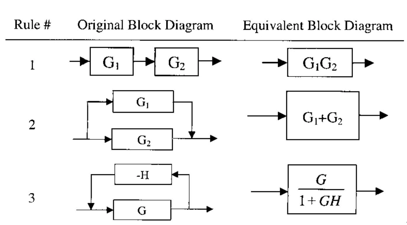
Transfer function with feedback is under form
G ( s ) 1 + G ( s ) H ( s ) \frac{G(s)}{1+G(s)H(s)} 1 + G ( s ) H ( s ) G ( s )
Equivalent Resistance and Impedance
x ˙ = A x + B u y = C x + D u \begin{align*}
\dot{x} &= Ax + Bu \\
y &= Cx + Du
\end{align*} x ˙ y = A x + B u = C x + D u
Given
G ( s ) = ∑ i = 1 n − 1 b i s i + b 0 s n + ∑ i = 1 n − 1 a i s i + a 0 = Y ( s ) U ( s ) G(s) = \frac{\sum_{i=1}^{n-1}b_is^i + b_{0}}{s^n + \sum_{i=1}^{n-1}a_is^{i} + a_{0}} = \frac{Y(s)}{U(s)} G ( s ) = s n + ∑ i = 1 n − 1 a i s i + a 0 ∑ i = 1 n − 1 b i s i + b 0 = U ( s ) Y ( s )
We get controller canonical state space form:
x ˙ ( t ) = [ 0 1 0 ⋯ 0 0 0 0 1 ⋯ 0 0 ⋮ ⋮ ⋮ ⋱ ⋮ ⋮ 0 0 0 ⋯ 1 0 0 0 0 ⋯ 0 1 − a 0 − a 1 − a 2 ⋯ − a n − 2 − a n − 1 ] x ( t ) + [ 0 0 ⋮ 0 0 1 ] u ( t ) y ( t ) = [ b 0 b 1 ⋯ b n − 2 b n − 1 ] x ( t ) . \begin{aligned}
\dot{x}(t) &= \begin{bmatrix}
0 & 1 & 0 & \cdots & 0 & 0 \\\
0 & 0 & 1 & \cdots & 0 & 0 \\\
\vdots & \vdots & \vdots & \ddots & \vdots & \vdots \\\
0 & 0 & 0 & \cdots & 1 & 0 \\\
0 & 0 & 0 & \cdots & 0 & 1 \\\
-a_0 & -a_1 & -a_2 & \cdots & -a_{n-2} & -a_{n-1}
\end{bmatrix} x(t) + \begin{bmatrix}
0 \\\
0 \\\
\vdots \\\
0 \\\
0 \\\
1
\end{bmatrix} u(t) \\\
y(t) &= \begin{bmatrix}
b_0 & b_1 & \cdots & b_{n-2} & b_{n-1}
\end{bmatrix} x(t).
\end{aligned} x ˙ ( t ) y ( t ) = 0 0 ⋮ 0 0 − a 0 1 0 ⋮ 0 0 − a 1 0 1 ⋮ 0 0 − a 2 ⋯ ⋯ ⋱ ⋯ ⋯ ⋯ 0 0 ⋮ 1 0 − a n − 2 0 0 ⋮ 0 1 − a n − 1 x ( t ) + 0 0 ⋮ 0 0 1 u ( t ) = [ b 0 b 1 ⋯ b n − 2 b n − 1 ] x ( t ) .
We get observer canonical state space form:
x ˙ ( t ) = [ − a n − 1 1 0 ⋯ 0 0 − a n − 2 0 1 ⋯ 0 0 ⋮ ⋮ ⋮ ⋱ ⋮ ⋮ − a 2 0 0 ⋯ 1 0 − a 1 0 0 ⋯ 0 1 − a 0 0 0 ⋯ 0 0 ] x ( t ) + [ b n − 1 b n − 2 ⋮ b 2 b 1 b 0 ] u ( t ) y ( t ) = [ 1 0 ⋯ 0 0 ] x ( t ) . \begin{aligned} \dot{x}(t) &= \begin{bmatrix} -a_{n-1} & 1 & 0 & \cdots & 0 & 0 \\ -a_{n-2} & 0 & 1 & \cdots & 0 & 0 \\ \vdots & \vdots & \vdots & \ddots & \vdots & \vdots \\ -a_2 & 0 & 0 & \cdots & 1 & 0 \\ -a_1 & 0 & 0 & \cdots & 0 & 1 \\ -a_0 & 0 & 0 & \cdots & 0 & 0 \end{bmatrix} x(t) + \begin{bmatrix} b_{n-1} \\ b_{n-2} \\ \vdots \\ b_2 \\ b_1 \\ b_0 \end{bmatrix} u(t) \\ y(t) &= \begin{bmatrix} 1 & 0 & \cdots & 0 & 0 \end{bmatrix} x(t). \end{aligned} x ˙ ( t ) y ( t ) = − a n − 1 − a n − 2 ⋮ − a 2 − a 1 − a 0 1 0 ⋮ 0 0 0 0 1 ⋮ 0 0 0 ⋯ ⋯ ⋱ ⋯ ⋯ ⋯ 0 0 ⋮ 1 0 0 0 0 ⋮ 0 1 0 x ( t ) + b n − 1 b n − 2 ⋮ b 2 b 1 b 0 u ( t ) = [ 1 0 ⋯ 0 0 ] x ( t ) .
See this for applications
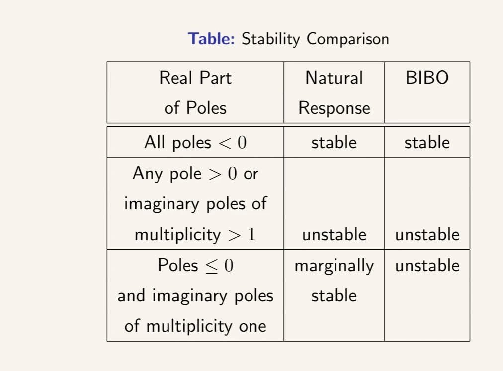
Necessary and sufficient condition for stability
to have all roots in open left hand plane is to have all coefficients of polynomial to be present and have same sign.
Routh table
To find transfer function for a system given a step response graph, *look for time over around 63% of the final value$
Closed-loop transfer function
T ( s ) = G ( s ) 1 + G ( s ) T(s) = \frac{G(s)}{1+G(s)} T ( s ) = 1 + G ( s ) G ( s )
%OS (percent overshoot)
% O S = e ζ π / 1 − ζ 2 × 100 % \%OS = e^{\zeta \pi / \sqrt{1-\zeta^2}} \times 100 \% % OS = e ζ π / 1 − ζ 2 × 100%
If a unity feedback system has a feedforward transfer function G ( s ) G(s) G ( s ) then transfer function E ( s ) R ( s ) \frac{E(s)}{R(s)} R ( s ) E ( s ) can be derived as:
C ( s ) = E ( s ) ⋅ G ( s ) E ( s ) = R ( s ) − C ( s ) \begin{aligned}
C(s) &= E(s)\cdot G(s) \\\
E(s) &= R(s) - C(s)
\end{aligned} C ( s ) E ( s ) = E ( s ) ⋅ G ( s ) = R ( s ) − C ( s )
For G ( s ) = K G(s) = K G ( s ) = K we get E ( s ) R ( s ) = 1 1 + G ( s ) \frac{E(s)}{R(s)} = \frac{1}{1+G(s)} R ( s ) E ( s ) = 1 + G ( s ) 1
state space design
Closed-loop system characteristic equation
d e t ( S I − ( A − B K ) ) det(SI - (A-BK)) d e t ( S I − ( A − B K ))
Gain and Phase Stability Margins
Closed loop pole exists when
1 + K G ( s ) H ( s ) = 0 1+KG(s)H(s) = 0 1 + K G ( s ) H ( s ) = 0
zero order hold
Nyqust frequency:
f N = 1 2 f s f_N = \frac{1}{2}f_s f N = 2 1 f s
Set the third pole to s=-2 to cancel a zero as third pole.