sparse crosscoders

maturity

a research preview from Anthroppic and this is pretty much still a work in progress

see also reproduction on Gemma 2B and github

A variant of sparse autoencoder where it reads and writes to multiple layers (Lindsey et al., 2024)

Crosscoders produces shared features across layers and even models

Resolve:

• cross-layer features: resolve cross-layer superposition

• circuit simplification: remove redundant features from analysis and enable jumping across training many uninteresting identity circuit connections

• model diffing: produce shared sets of features across models. This also introduce one model across training, and also completely independent models with different architectures.

motivations

cross-layer superposition

given the additive properties of transformers’ residual stream, adjacent layers in larger transformers can be thought as “almost parallel”

intuition

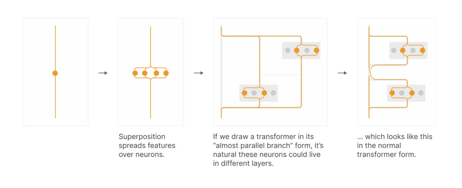
In basis of superposition hypothesis, a feature is a linear combinations of neurons at any given layers.

if we think of adjacent layers as being “almost parallel branches that potentially have superposition between them”, then we can apply dictionary learning jointly ¹

persistent features and complexity

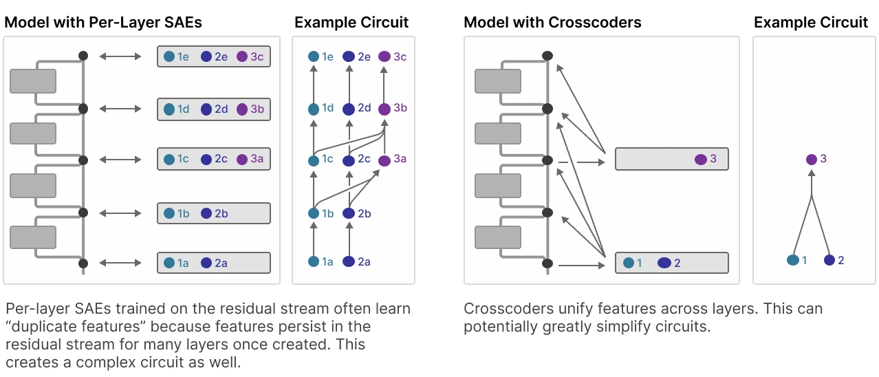
Current drawbacks of sparse autoencoders is that we have to train it against certain activations layers to extract features. In terms of the residual stream per layers, we end up having lots of duplicate features across layers.

Crosscoders can simplify the circuit given that we use an appropriate architecture ²

setup.

Autoencoders and transcoders as special cases of crosscoders.

• autoencoders: reads and predict the same layers
• transcoders: read from layer $n$ and predict layer $n+1$

Crosscoder read/write to many layers, subject to causality constraints.

definition

Let one compute the vector of feature activation $f_{(}{x}_j)$ on datapoint $x_j$ by summing over contributions of activations of different layers $a^l(x_j)$ for layers $l\in L$:

$$\begin{array}{rl}f(x_j)& =\text{ReLU}(\sum _{l\in L}{W}_{\text{enc}}^l{a}^l(x_j)+b_{\text{enc}})\\ & \\ & \because W_{\text{enc}}^l:\text{ encoder weights at layer }l\\ & \\ & \because a^l(x_j):\text{ activation on datapoint }{x}_j\text{ at layer }l\end{array}$$

We have loss

$$L=\sum _{l\in L}\Vert a^l(x_j)-a^{l^{{}^{\prime }}}(x_j){\Vert }^2+\sum _{l\in L}\sum _i{f}_i(x_j)\Vert W_{\text{dec,i}}^l\Vert$$

and regularization can be rewritten as:

$$\sum _{l\in L}\sum _i{f}_i(x_j)\Vert W_{\text{dec,i}}^l\Vert =\sum _i{f}_i(x_j)(\sum _{l\in L}\Vert W_{\text{dec,i}}^l\Vert )$$

weight of L1 regularization penalty by L1 norm of per-layer decoder weight norms $\sum l\in L\Vert W_{\text{dec,i}}^l\Vert$ ³

We use L1 due to

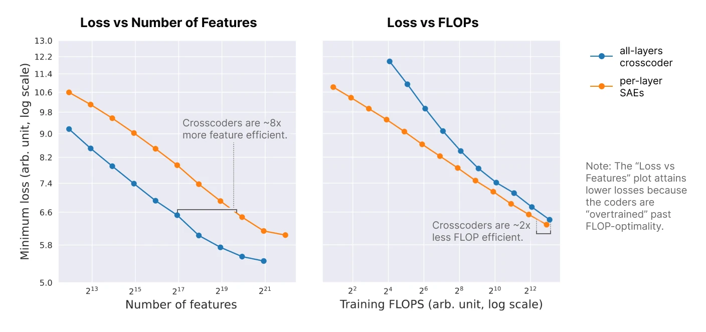
• baseline loss comparison: L2 exhibits lower loss than sum of per-layer SAE losses, as they would effectively obtain a loss “bonus” by spreading features across layers

• layer-wise sparsity surfaces layer-specific features: based on empirical results of model diffing, that L1 uncovers a mix of shared and model-specific features, whereas L2 tends to uncover only shared features.

variants

good to explore:

1. strictly causal crosscoders to capture MLP computation and treat computation performed by attention layers as linear
2. combine strictly causal crosscoders for MLP outputs without weakly causal crosscoders for attention outputs
3. interpretable attention replacement layers that could be used in combination with strictly causal crosscoders for a “replacement model”

model diffing

see also: model stiching and SVCCA

(Laakso & Cottrell, 2000) proposes compare representations by transforming into representations of distances between data points. ⁴

questions

How do features change over model training? When do they form?

As we make a model wider, do we get more features? or they are largely the same, packed less densely?

Gorton, L. (2024). The Missing Curve Detectors of InceptionV1: Applying Sparse Autoencoders to InceptionV1 Early Vision. arXiv preprint arXiv:2406.03662 arxiv

Laakso, A., & Cottrell, G. (2000). Content and cluster analysis: Assessing representational similarity in neural systems. Philosophical Psychology, 13(1), 47–76. https://doi.org/10.1080/09515080050002726

Lindsey, J., Templeton, A., Marcus, J., Conerly, T., Batson, J., & Olah, C. (2024). Sparse Crosscoders for Cross-Layer Features and Model Diffing. Transformer Circuits Thread. [link]

Footnotes

1. (Gorton, 2024) applies SAEs to study InceptionV1, where cross-branch superposition is significant in interpreting models with parallel branches ↩

2. causal description it provides likely differs from that of the underlying model. ↩

3. $\Vert W_{\text{dec,i}}^l\Vert$ is the L2 norm of a single feature’s decoder vector at a given layer.

   In principe, one might have expected to use L2 norm of per-layer norm $\sqrt{{\sum }_{l\in L}\Vert W_{\text{dec,i}}^l{\Vert }^2}$ ↩

4. Chris Colah’s blog post explains how t-SNE can be used to visualize collections of networks in a function space. ↩