⌘ '

raccourcis clavier

Real-time control systems, and scheduling

time domain versus frequency domain

use Laplace transform to convert from time domain to frequency domain

Consider the following circuit:

\begin{aligned} \text{RC} \frac{d v_o(t)}{dt} + v_o(t) &= v_i(t) \\ v_i(t) &= 1 \end{aligned}

graph LR
    Diff{{differential equations}} -- "Laplace transform" --> Algebraic{{algebraic equations}} -- "inverse Laplace transform" --> End{{time domain solution}}

\mathcal{L} \{f(t)\} = \int_0^{\infty}f(t)^{-st}dt = F(s)

\begin{array}{c c c} \hline \text{Item no.} & f(t) & F(s) \\ \hline 1. & \delta(t) & 1 \\ 2. & u(t) & \frac{1}{s} \\ 3. & tu(t) & \frac{1}{s^2} \\ 4. & t^n u(t) & \frac{n!}{s^{n+1}} \\ 5. & e^{-at}u(t) & \frac{1}{s + a} \\ 6. & \sin(\omega t)u(t) & \frac{\omega}{s^2 + \omega^2} \\ 7. & \cos(\omega t)u(t) & \frac{s}{s^2 + \omega^2} \\ \hline \end{array}

\delta{(t)} = 0, \quad t \neq 0,\quad \int_0^{\infty}{\delta{(t)}}dt=1

example: Given a unit step function $u(t) = \begin{cases} 0 & t < 0 \\ 1 & t \ge 0 \end{cases}$

\begin{aligned} U(s) = \mathcal{L} \{u(t)\} &= \int_{0}^{\infty} u(t) e^{-st} dt = -\frac{1}{s} e^{-st} dt \\ U(s) &= -\frac{1}{s}(0-1) = \frac{1}{s} \end{aligned}

inverse form

\mathcal{L}^{-1} \{ F(s) \} = \frac{1}{2\pi j} \lim_{\omega \to \infty} \int_{\sigma-j\omega}^{\sigma+j\omega} F(s) e^{st} \, ds

derivatives and integral

if $\mathcal{L}[f(t)] = F(s)$ then we have
$\begin{aligned} \mathcal{L}[f^{'}(t)] &= sF(s) -f(0) \\ \mathcal{L}[\int_0^{t}f(t) dt] &= \frac{F(s)}{s} \end{aligned}$

For higher derivatives we have $\mathcal{L}[f^{''}(t)] = s^{2} F(s) - sf(0) - f^{'}(0)$

another form of system model

we can replace $s$ with $jw$

ex: $G(jw) = \frac{1}{1+jw \text{RC}}$ , so $|G(jw)| = |\frac{1}{1+jw \text{RC}}| = \frac{1}{\sqrt{1+(w \text{RC}^2)}}$

reasoning: we substitute Laplace transform with Fourier transform with $s=jw$

example for a first-order system

\begin{aligned} Y(s) &= \frac{s+2}{s(s+5)} = \frac{2}{5s} + \frac{3}{5(s+5)} \\ y(t) &= \frac{2}{5} + \frac{3}{5} e^{-5t} \\[8pt] \because \text{total response} &= \text{forced} + \text{natural} \end{aligned}

stability: total response = natural response + forced response

the output response of a system

natural (transient) response: $\frac{3}{5} e^{-5t}$

forced response (steady-state) response: $\frac{2}{5}$

poles and zeros

zeros and poles generate the amplitude for both forced and natural response

Y(s) = \frac{s+2}{s(s+5)}

$s=0,-5$ are poles and $s=-2$ are zeros

poles

at origin, generated step function

at -5 generate transient response $e^{-5t}$

We will consider first-order and second-order system

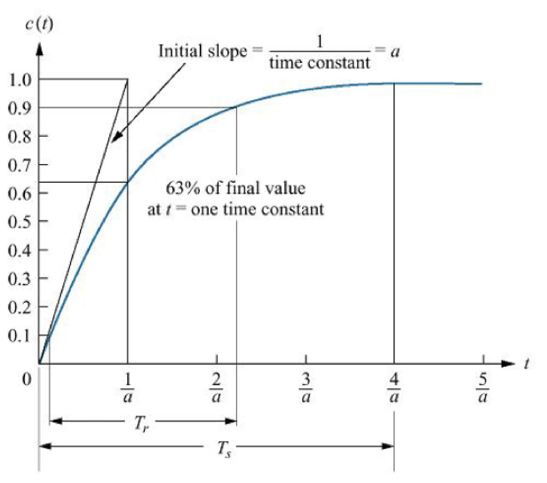
first-order systems, time constant

"\\usepackage{tikz}\n\\usetikzlibrary{positioning}\n\n\\begin{document}\n\\begin{tikzpicture}[auto, node distance=2cm, >=latex]\n\n% Nodes\n\\node[draw, rectangle, minimum width=3cm, minimum height=1.5cm] (block) {$\\frac{a}{s + a}$};\n\\node[left=1.5cm of block] (input) {$X(s) = \\frac{1}{s}$};\n\\node[right=1.5cm of block] (output) {$Y(s)$};\n\\node[above=0.5cm of block] (G) {$G(s)$};\n\n% Arrows\n\\draw[->] (input) -- (block);\n\\draw[->] (block) -- (output);\n\n\\end{tikzpicture}\n\\end{document}"

source code

Output of a general first-order system is

Y(s) = X(s)G(s) = \frac{a}{s(s+a)}

thus the time domain output is $y(t) = 1 - e^{-at}$

time constant

usually, $t=\frac{1}{a}$ , and $y(t) = 0.63$ , hence 63.2% to find the rise time.

response in time domain

rise time $T_r$

$T_r$ , time for the waveform to go from 0.1 to 0.8 of its final value

for first order: $T_r = \frac{2.2}{a}$

settling time $T_s$

$T_s$ , time for response to reach and stay with 2% of its final value

for first order: $T_s = \frac{4}{a}$

second-order systems

general order system:

G(s) = \frac{b}{s^{2}+as +b}

Thus the pole for this system:

s_{1},s_{2}= \frac{-a + \sqrt{a^2 - 4b}}{2}

natural frequency

happens when $a=0$

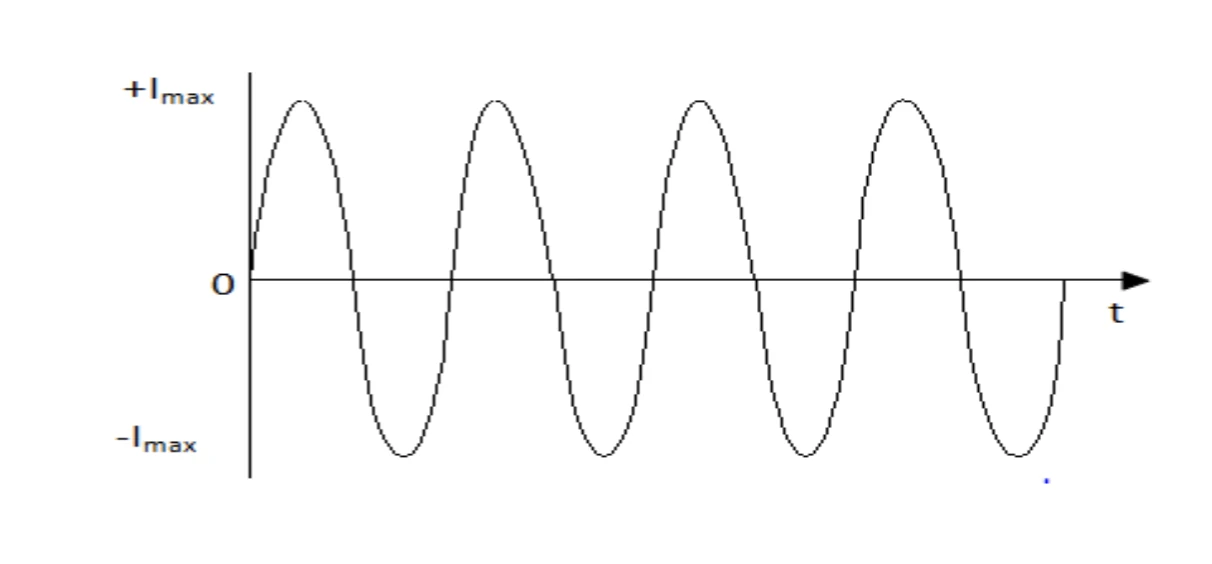
The transfer function is $G(s)=\frac{b}{s^{2}+b}$ , and poles will only have imaginary $\pm jw$

$w_n = \sqrt{b}$ is the frequency of oscillation of this system.

in a sense, this is the undamped case:

damping coefficient

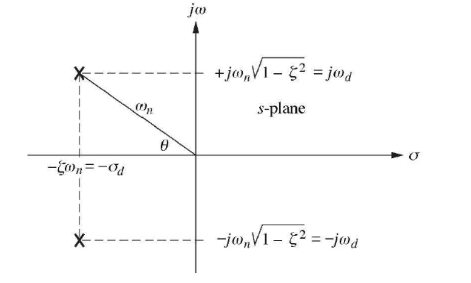
complex poles has real part $\sigma = -\frac{a}{2}$

definition

damping ratio is defined as:
$\zeta = \frac{\text{exponential decay frequency}}{\text{natural frequency}} = \frac{|\sigma|}{w_n}$

So that $a = 2 \zeta w_n$

general second order

\begin{aligned} G(s) &= \frac{w_n^2}{s^2 + 2 \zeta w_n s + w_n^2} \\[12pt] s_{1},s_{2} &= - \zeta w_n \pm w_n \sqrt{\zeta^2 - 1} \end{aligned}

observations

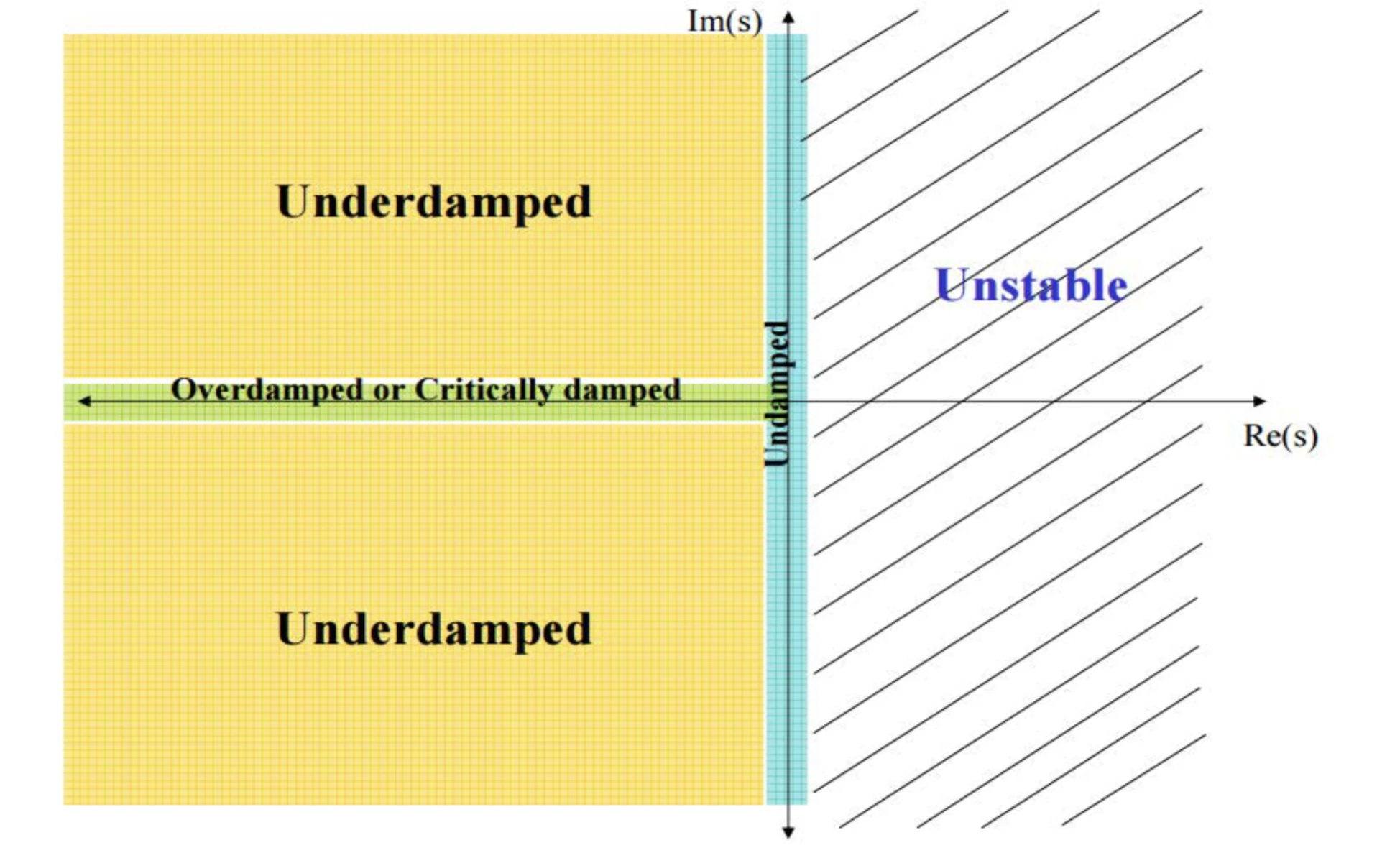
Condition	Poles	pole type	Damping Ratio ( $\zeta$ )	Natural Response $c(t)$
Undamped	$\pm j \omega_n$	imaginary	$\zeta = 0$	$A \cos (\omega_n t - \varphi)$
Underdamped	$\omega_d \pm j \omega_d$	complex	$0 < \zeta < 1$	$A e^{(-\sigma_d)t} \cos (\omega_d t - \varphi)$ where $w_d = w_n \sqrt{1- \zeta^2}$
critically damped	$\sigma_1$	real	$\zeta = 1$	$K t e^{\sigma_1 t}$
overdamped	$\sigma_1 \quad \sigma_2$	real	$\zeta > 1$	$K (e^{\sigma_1 t} + e^{\sigma_2 t})$

underdamped second-order step response

Transfer function $C(s)$ is given by

C(s) = \frac{w_n^2}{s(s^2 + 2 \zeta w_n s + w_n^2)}

response in time-domain via inverse Laplace transform:

c(t) = 1 - \frac{1}{\sqrt{1- \zeta^2}} e^{- \zeta w_n t} \cos (\sqrt{1- \zeta^2}\omega_n t + \varphi)

where $\varphi = \tan^{-1} (\frac{\zeta}{\sqrt{1-\zeta^2}})$

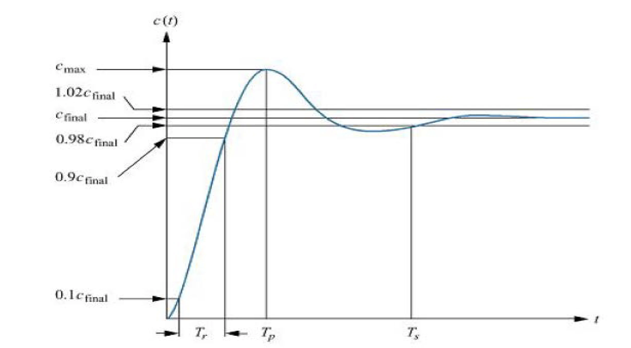
peak time $T_p$

time required to reach the first or maximum peak

T_p = \frac{\pi}{\omega_n \sqrt{1-\zeta^2}}

percent overshoot

%OS (percent overshoot)

\%OS = e^{\zeta \pi / \sqrt{1-\zeta^2}} \times 100 \%

or in terms of damping ratio $\zeta$ :

\zeta = \frac{-\ln \frac{\text{\%OS}}{100}}{\sqrt{\pi^2 + \ln^2(\frac{\text{\%OS}}{100})}}

relations to poles

\begin{aligned} G(s) &= \frac{w_n^2}{s^2 + 2 \zeta w_n s + w_n^2} \\[12pt] s_{1},s_{2} &= - \zeta w_n \pm w_n \sqrt{\zeta^2 - 1} \\[8pt] T_p &= \frac{\pi}{\omega_n \sqrt{1-\zeta^2}} \\ T_s &\cong \frac{4}{\zeta \omega_n} \end{aligned}

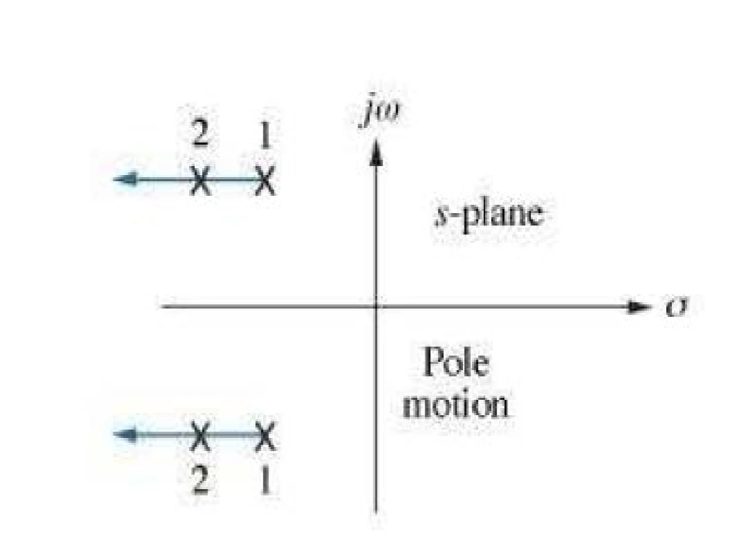
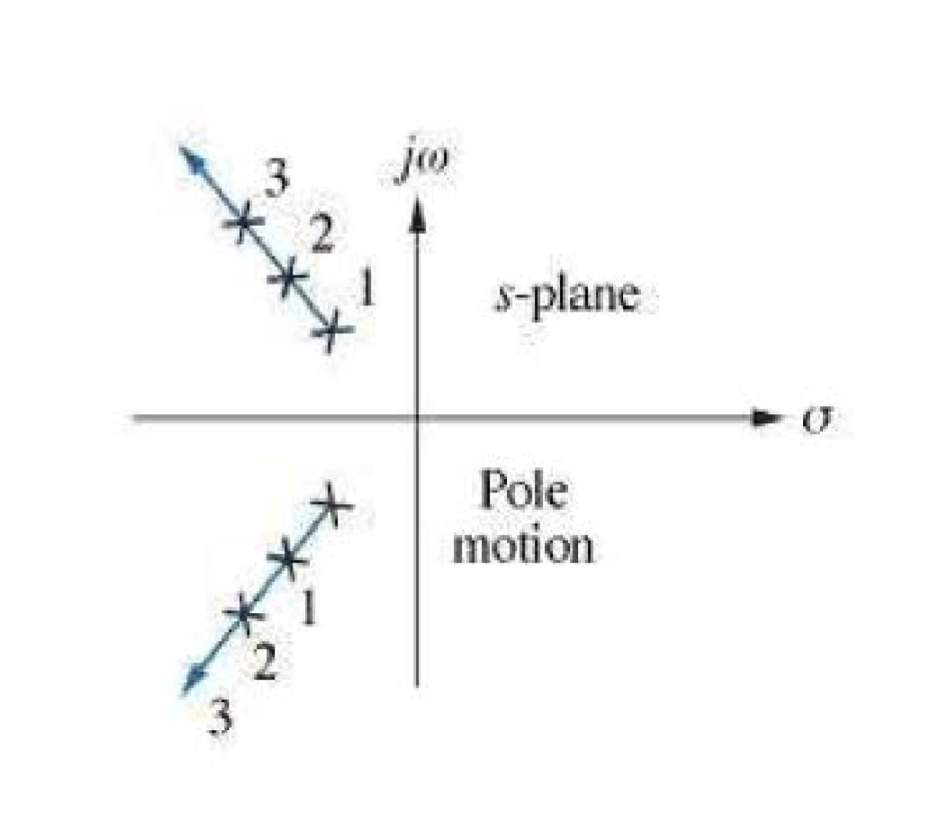
poles of second-order underdamped system

location of poles	response	examples
Same envelope		system response
Same frequency		system response
Same overshoot		system response

same envelope

"\\usepackage{tikz}\n\\usepackage{pgfplots}\n\\pgfplotsset{compat=1.16}\n\n\\begin{document}\n\\begin{tikzpicture}\n \\begin{axis}[\n width=12cm, height=8cm,\n xlabel={$t$ (time)},\n ylabel={Amplitude},\n grid=major,\n legend style={at={(0.5,1.1)}, anchor=north, legend columns=-1},\n xmin=0, xmax=10,\n ymin=-1.2, ymax=1.2\n ]\n % First Transfer Function (Sinusoidal)\n \\addplot[blue, thick, samples=100, domain=0:10]\n {exp(-0.1*x)*sin(deg(2*pi*0.5*x))};\n\n % Second Transfer Function (Envelope with Different Frequency)\n \\addplot[red, dashed, thick, samples=100, domain=0:10]\n {exp(-0.1*x)*sin(deg(2*pi*0.8*x))};\n\n % Envelope (Exponential Decay)\n \\addplot[black, dotted, thick, samples=100, domain=0:10]\n {exp(-0.1*x)};\n\n \\addplot[black, dotted, thick, samples=100, domain=0:10]\n {-exp(-0.1*x)};\n \\end{axis}\n\\end{tikzpicture}\n\\end{document}"

source code

same frequency

"\\usepackage{tikz}\n\\usepackage{pgfplots}\n\\pgfplotsset{compat=1.16}\n\n\\begin{document}\n\\begin{tikzpicture}\n \\begin{axis}[\n width=12cm, height=8cm,\n xlabel={$t$ (time)},\n ylabel={Amplitude},\n grid=major,\n legend style={at={(0.5,1.1)}, anchor=north, legend columns=-1},\n xmin=0, xmax=10,\n ymin=-3, ymax=3\n ]\n % First Transfer Function (Higher Amplitude)\n \\addplot[blue, thick, samples=100, domain=0:10]\n {2*sin(deg(2*pi*0.5*x))};\n\n % Second Transfer Function (Lower Amplitude)\n \\addplot[red, dashed, thick, samples=100, domain=0:10]\n {1*sin(deg(2*pi*0.5*x))};\n \\end{axis}\n\\end{tikzpicture}\n\\end{document}"

source code

same overshoot

"\\usepackage{tikz}\n\\usepackage{pgfplots}\n\\pgfplotsset{compat=1.16}\n\n\\begin{document}\n\\begin{tikzpicture}\n \\begin{axis}[\n width=12cm, height=8cm,\n xlabel={Time $t$},\n ylabel={Response},\n grid=major,\n legend style={at={(0.5,1.1)}, anchor=north, legend columns=-1},\n xmin=0, xmax=10,\n ymin=0, ymax=2\n ]\n % First System Response\n \\addplot[blue, thick, samples=200, domain=0:10]\n {1 - exp(-0.5*x)*(cos(deg(2*pi*0.5*x)) + 0.1*sin(deg(2*pi*0.5*x)))};\n\n % Second System Response (Same Overshoot, Different Natural Frequency)\n \\addplot[red, dashed, thick, samples=200, domain=0:10]\n {1 - exp(-1*x)*(cos(deg(2*pi*1*x)) + 0.05*sin(deg(2*pi*1*x)))};\n\n % Reference Line for Steady-State Response\n \\addplot[black, dotted, thick] coordinates {(0,1) (10,1)};\n \\end{axis}\n\\end{tikzpicture}\n\\end{document}"

source code

reference: slides, and awesome calculator

excerpt from real-time system slides

final value theorem

If a system is stable and has a final constant value, then one can find steady state value without solving for system’s response. Formally:
$\lim_{t \to \infty} x(t) = \lim_{s \to 0} sX(s)$

sketching root locus

Rule	Description
Number of Branches	Number of closed-loop poles, or the number of finite open-loop poles = number of finite open-loop zeros
Symmetry	About the real axis
Start and End Points	Starts at poles of open loop transfer function and ends at finite and infinite open loop zeros
Behaviour at $\infty$	Real axis: $\sigma_a = \frac{\Sigma{\text{finite poles}} - \Sigma{\text{finite zeros}}}{\text{\# finite poles - \# finite zeros}}$ Angle: $\theta_a = \frac{(2k+1)\pi}{\text{\# finite poles - \# finite zeros}}$ where $k = 0, \pm 1, \pm 2, \pm 3$
Breakaway/Break-in Points	Located at roots where $\frac{d[G(s)H(s)]}{ds} = 0$

Control Type	Transfer function $T(s)$	Key Characteristics	Effects
Proportional (P)	$\frac{K_p G_p}{1 + K_p G_p}$	Basic control action	- Affects speed of response - Cannot eliminate steady-state error
Integral (I)	$\frac{K_I}{s^2 + s + K_I}$	Integrates error over time	- Eliminates steady-state error - Output reaches 1 at steady state
PI	$\frac{K_I + sK_p}{s^2 + (1+K_p)s + K_I}$	Combines P and I	- P impacts response speed - I forces zero steady-state error
Derivative (D)	$\frac{K_D s}{(1+K_D)s + 1}$	Based on rate of change	- Adds open-loop zero - Can affect stability - Provides damping effect

PID control

G_C(s) = K_p + \frac{K_I}{s} + K_D s

in time domain:

u(t) = K_P e(t) + K_I \int_{0}^{t} e(\eta) d\eta + K_D \frac{d(e(t))}{dt}

Component	Discrete-Time Equation
Proportional	$u(k) = K_P e(k)$
Integral	$u(k) = K_I T \sum_{i=1}^{k} e(i)$
Derivative	$u(k) = \frac{K_D}{T}[e(k) - e(k-1)]$

approximate of PID controller: $u(k) = K_P e(k) + K_I T \sum_{i=1}^{n} e(i) + \frac{K_D}{T}[e(k) - e(k-1)]$

S and Z-transform table

Time Domain $x(t)$	Laplace Transform $X(s)$	Z Transform $X(z)$
$\delta(t) = \begin{cases} 1 & t = 0 \\ 0 & t = kT, k \neq 0 \end{cases}$	$1$	$1$
$\delta(t - kT) = \begin{cases} 1 & t = kT \\ 0 & t \neq kT \end{cases}$	$e^{-kTs}$	$z^{-k}$
$u(t)$ (unit step)	$\frac{1}{s}$	$\frac{z}{z - 1}$
$t$	$\frac{1}{s^2}$	$\frac{Tz}{(z - 1)^2}$
$t^2$	$\frac{2}{s^3}$	$\frac{T^2 z(z + 1)}{(z - 1)^3}$
$e^{-at}$	$\frac{1}{s + a}$	$\frac{z}{z - e^{-aT}}$
$1 - e^{-at}$	$\frac{a}{s(s + a)}$	$\frac{(1 - e^{-aT})z}{(z - 1)(z - e^{-aT})}$
$te^{-at}$	$\frac{1}{(s + a)^2}$	$\frac{Tz e^{-aT}}{(z - e^{-aT})^2}$
$t^2 e^{-at}$	$\frac{2}{(s + a)^3}$	$\frac{T^2 e^{-aT} z(z + e^{-aT})}{(z - e^{-aT})^3}$
$b e^{-bt} - a e^{-at}$	$\frac{(b - a)s}{(s + a)(s + b)}$	$\frac{z [ z(b - a) - (b e^{-aT} - a e^{-bT}) ]}{(z - e^{-aT})(z - e^{-bT})}$
$\sin \omega t$	$\frac{\omega}{s^2 + \omega^2}$	$\frac{z \sin \omega T}{z^2 - 2z \cos \omega T + 1}$
$\cos \omega t$	$\frac{s}{s^2 + \omega^2}$	$\frac{z(z - \cos \omega T)}{z^2 - 2z \cos \omega T + 1}$
$e^{-at} \sin \omega t$	$\frac{\omega}{(s + a)^2 + \omega^2}$	$\frac{z e^{-aT} \sin \omega T}{z^2 - 2z e^{-aT} \cos \omega T + e^{-2aT}}$

reference: examples for z-transform

Sequence	Transform
$\delta(k - n)$	$z^{-n}$
$1$	$\frac{z}{z - 1}$
$k$	$\frac{z}{(z - 1)^2}$
$k^2$	$\frac{z(z + 1)}{(z - 1)^3}$
$a^k$	$\frac{z}{z - a}$
$ka^k$	$\frac{az}{(z - a)^2}$
$\sin ak$	$\frac{z \sin a}{z^2 - 2z \cos a + 1}$
$\cos ak$	$\frac{z(z - \cos a)}{z^2 - 2z \cos a + 1}$
$a^k \sin bk$	$\frac{az \sin b}{z^2 - 2az \cos b + a^2}$
$a^k \cos bk$	$\frac{z^2 - az \cos b}{z^2 - 2az \cos b + a^2}$

properties

Linearity: if $x(n) = af_{1}(n) + bf_{2}(n)$ then $X(z) = aF_{1}(z) + bF_{2}(z)$

Time shifting:

\begin{aligned} Z[x(t)] &= X(z) \\ x(k-n) &= z^{-n}X(z) \\ x(k+n) &= z^{n}X(z) \end{aligned}

quantization error

sampling

The idea to convert analog to digital

$T$ is the sampling period, and $\frac{1}{T}$ is the sampling rate in cycles per second

\text{error} = \frac{M}{2^{n+1}}

where $n$ is number of bits used for digitalisation

resolution of A/D converter

minimum value of the output that can be represented as binary number, or $\frac{M}{2^n}$

sampled data system

reference input $r$ is the sequence of sample values $r(kT)$

A sampler is a switch that closes every $T$ seconds:

r^{*}(t) = \sum_{k=0}^{\infty} r(kT) \delta (t-kT) \quad (t>0)

Transfer function of sampled data:

R^{*}(s) = \mathcal{L} (r^{*}(t)) = \sum_{k=0}^{\infty} r(kT) e^{-ksT}

definition

Let $z = e^{sT}$ , we have the following definition:

z-transform

$Z \{r(t)\} = F(z) = Z(r^{*}(t)) = \sum_{k=0}^{\infty} r(kT)z^{-k}$

zero-order hold

Transfer function of Zero-Order hold

\mathcal{L}(u(t) - u(t-T)) = \frac{1}{s} - \frac{e^{sT}}{s}

finding the discrete transfer function

$G(s) = \frac{s^2 + 4s + 3}{s^3 + 6s^2 + 8s}$

\begin{aligned} G(s) &= \frac{s^2 + 4s + 3}{s^3 + 6s^2 + 8s} = \frac{0.375}{s} + \frac{0.25}{s+2} + \frac{0.375}{s+4} \\ G(t) &= \mathcal{L}^{-1}(G(s)) = 0.375 + 0.25 e^{-2t} + 0.375 e^{-4t} \\ G(z) &= Z(G(t)) = 0.375 \frac{z}{z-1} + 0.25 \frac{z}{z-e^{-2T}} + 0.375 \frac{z}{z-e^{-4T}} \end{aligned}

inverse z-transform

$G(z) \to x(k)$

power series

use: when G(z) is expressed as the ratio of two polynomials in z

G(z) = a_{0} + a_{1} z^{-1} + a_{2} z^{-2} + \ldots

partial fraction

For example: $G(z) = \frac{z}{(z-1)(z-2)} = \frac{-z}{z-1} + \frac{z}{z-2} = \sum_{k=0}^{\infty} (-1 + 2^k)z^{-k}$

thus, $g(kT) = 2^k-1$

stability

system	pole location criteria on z-plane
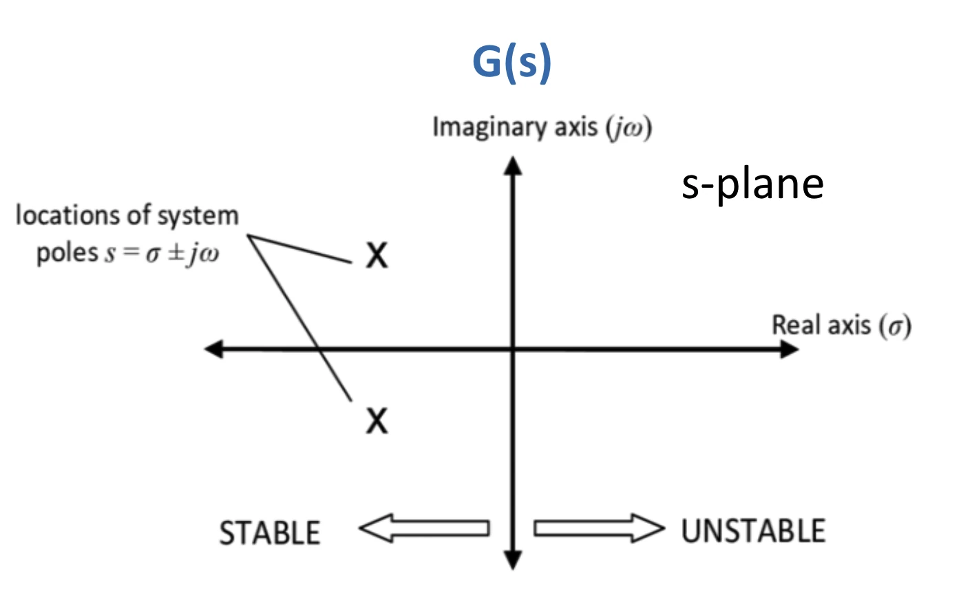
Stable	All poles inside unit circle
Unstable	Any poles outside unit circle
Marginally Stable	One or more poles on unit circle, remaining poles inside unit circle

poles on s-plane

mapping from s-plane to z-plane

$z = e^{\alpha T}(\cos \omega T + j \sin \omega T)$

we assume $s = \alpha + j \omega$

Location on s-plane	Value of $\alpha$	Value of $e^{\alpha T}$	Mapping on z-plane
Imaginary axis ( $j\omega$ )	$\alpha = 0$	$e^{\alpha T} = 1$	On unit circle
Right half-plane	$\alpha > 0$	$e^{\alpha T} > 1$	Outside unit circle
Left half-plane	$\alpha < 0$	$e^{\alpha T} < 1$	Inside unit circle

final value theorem

definition

If $\lim_{k \to \infty}x(k)$ exists, then the follow exists:
$\lim_{k \to \infty} x(k) = \lim_{z \to 1} (z-1) X(z)$

root locus on z-plane

derive open loop function $K \bar{GH}$
Factor numerator and denominator to get open loop zeros and poles
Plot roots of $1+K \bar{GH}=0$ in z-plane as k varies $\bar{GH(z)} = \frac{N(z)}{D(z)}$

For determine discrete systems and vice versa.

$G(z)$ with a Zero-Order hold

G(z) = (1-z^{-1}) Z[\frac{G_p(s)}{s}] = G^{*}(z) - z^{-1}G^{*}(z)

example: Find $G(z)$ if $G_p(s) = \frac{s+2}{s+1}$

\begin{aligned} G^{*}(s) &= \frac{G_p(s)}{s} = \frac{2}{s} - \frac{1}{s+1} \\[8pt] g^{*}(t) &= 2 - e^{-t} \quad (\text{inverse Laplace transform}) \\ g^{*}(kT) &= 2 - e^{-kT} \\ G^{*}(z) = \frac{2z}{z-1} - \frac{z}{z-e^{-T}} \end{aligned}

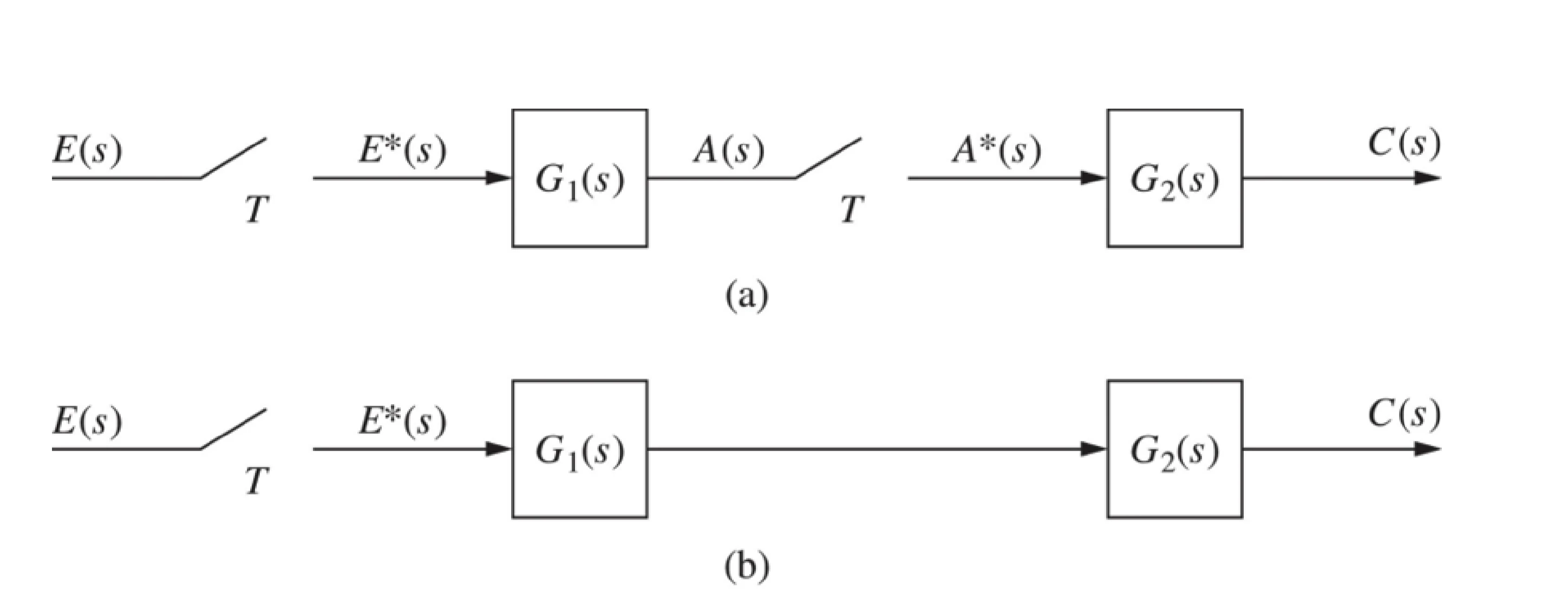
block diagram reduction

a. $C(z) = G_1(z) G_2(z) E(z)$ b. $C(z) = Z[G_1(s) G_2(s)]E(z)$

Note

The product of $G_1(s)G_2(s)$ must be evaluated first

model for Open-loop system

The output of open-loop system is

C(z) = G(z)D(z)E(z)

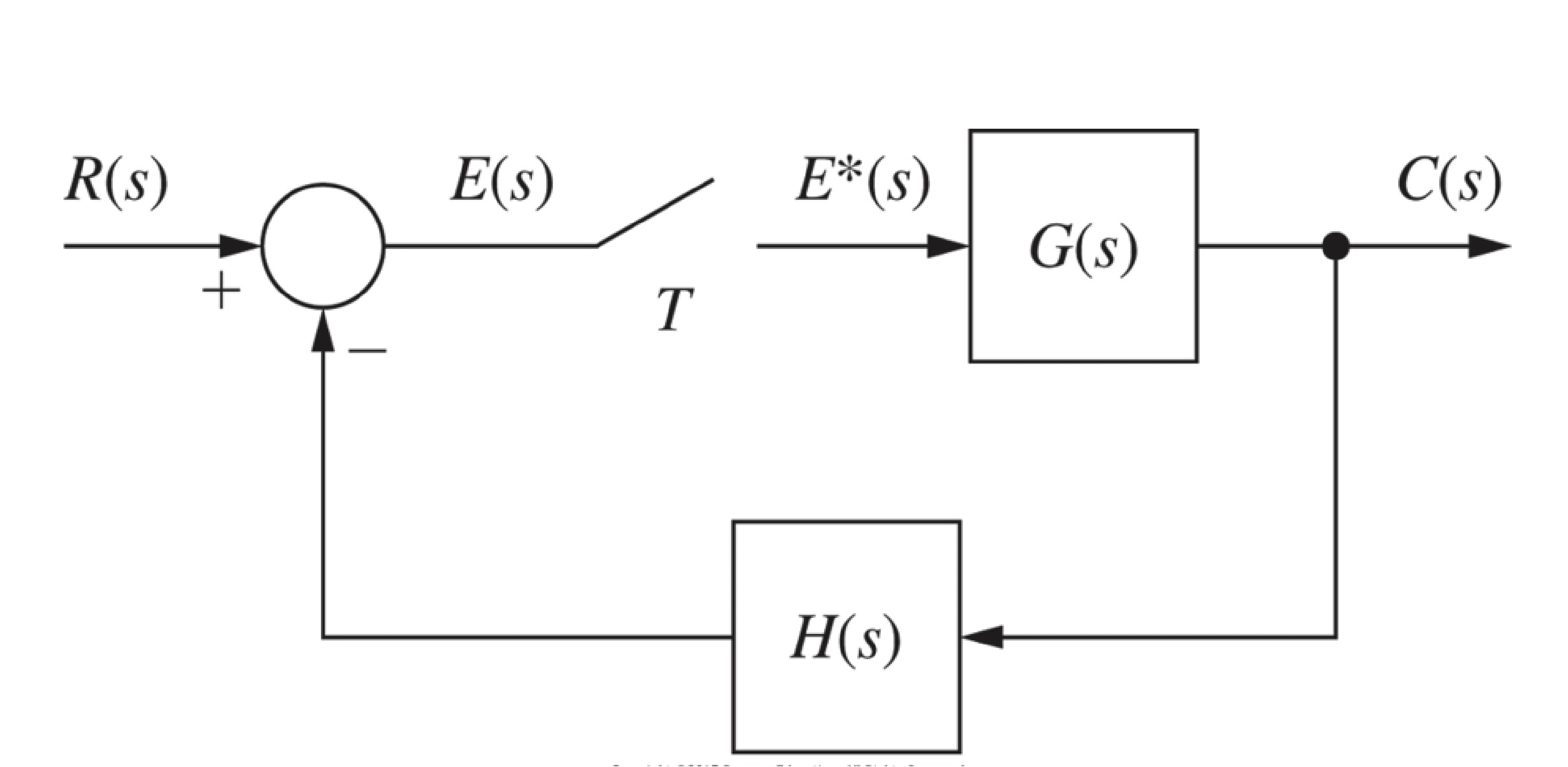
closed loop sample data system

\begin{aligned} E(z) &= R(z) - Z[G(s)H(s)]E(z) \\[12pt] &\because \frac{C(z)}{R(z)} = \frac{G(z)}{1+Z[G(s)H(s)]} \end{aligned}

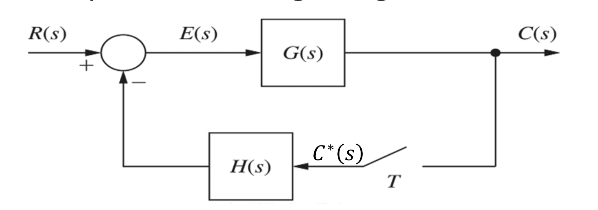
using digital sensing device

C(z) = \frac{Z[G(s)R(s)]}{1+Z(G(s)H(s))}

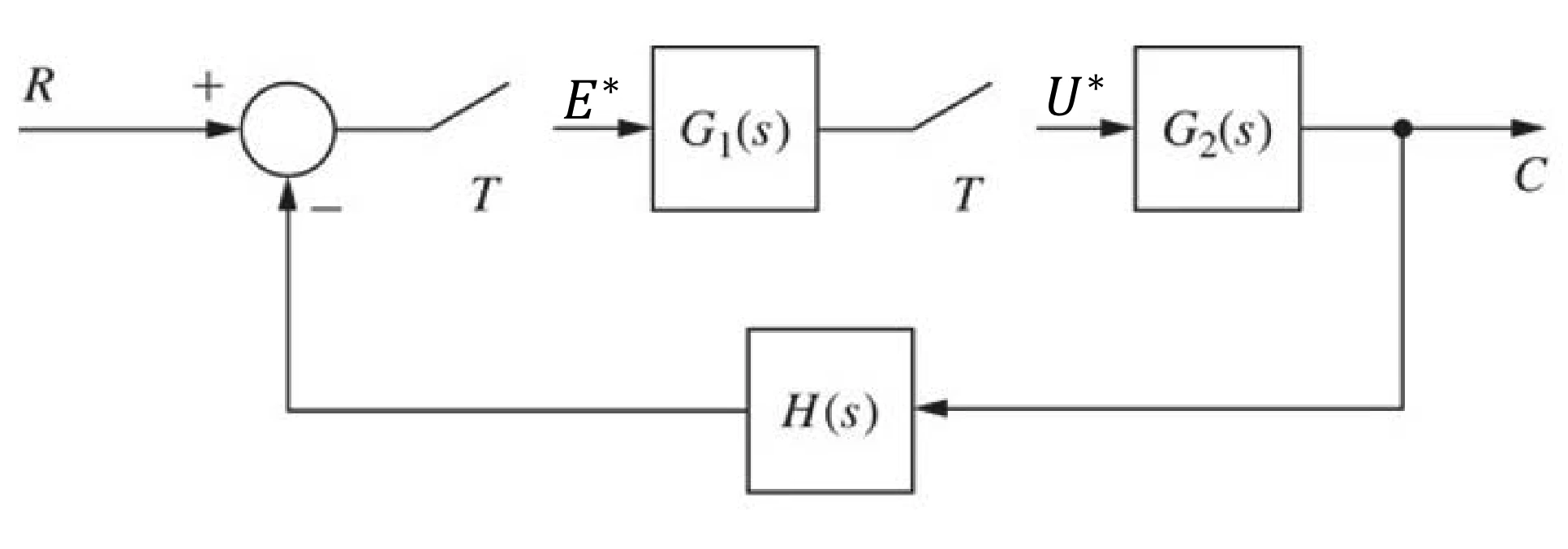
using digital controller

\frac{C(z)}{R(z)} = \frac{G_{1}(z)G_{1}(z)}{1+G_{1}(z)Z(G_{2}(s)H(s))}

time response

T(z) = \frac{G(z)}{1+G(z)}

System Type	Transfer Function	Diagram
Basis	$\frac{C(z)}{R(z)} = \frac{G(z)}{1+Z[G(s)H(s)]}$
w/ digital sensing device	$C(z) = \frac{Z[G(s)R(s)]}{1+Z(G(s)H(s))}$
w/ digital controller	$\frac{C(z)}{R(z)} = \frac{G_{1}(z)G_{1}(z)}{1+G_{1}(z)Z(G_{2}(s)H(s))}$

Assume the transfer function is given by

D(s) = \frac{U(s)}{E(s)} = K_{0} \frac{s+a}{s+b}

difference equation

$u(k) = (1-bT)u(k-1) + K_{0}(aT-1)E(k-1) + K_{0}e(k)$

The corresponding z-transform

\begin{aligned} \frac{U(z)}{E(z)} &= \frac{K_{0}(aT-1)z^{-1} + K_{0}}{1+(bT-1)z^{-1}} = \frac{K_{0}z + K_{0}(aT-1)}{z+(bT-1)} \\ &=[K_{0}(aT-1) + zK_{0}]/[z+(bT-1)] \end{aligned}

z-transform of difference equation

example: Given $D(s) = \frac{a}{s+a}$ , $u(kT) = u(k)$

$U(s)(s+a) = aE(s)$ (Laplace transform) gives $\frac{u(k+1)-u(k)}{T} + au(k) = a e(k)$

difference equation is $u(k+1) = (1-aT)u(k) + aTe(k)$

z-transform is $\frac{U(z)}{E(z)}=\frac{aT z^{-1}}{1+(aT -1)z^{-1}}=\frac{aT}{z+(aT-1)}$

discrete equivalent

Consider the example

\begin{aligned} D(s) &= \frac{U(s)}{E(s)} = \frac{a}{s+a} \to U(s)s = aE(s) - aU(s) \\ &\to u^{'}(t) = -au(t) + ae(t) \end{aligned}

u(t) = \int_0^t [-au(\tau) + ae(\tau)] d \tau

for discrete system

$u(kT) = u(kT - T) + \int_{kT-T}^{kT} [-au(\tau) + ae(\tau)] d \tau$

We can use the following approximation methods for the second term from $D(z)$ to $D(s)$

$D(s)$	rule	z-transfer function $D(z)$	approximation	z-plane to s-plane	stability
$\frac{a}{s+a}$	forward	$\frac{a}{(z-1)/T+a}$	$s \gets \frac{z-1}{T}$	$z \gets sT + 1$	discrete $\to$ continuous
$\frac{a}{s+a}$	backward	$\frac{a}{(z-1)/(Tz)+a}$	$s \gets \frac{z-1}{Tz}$	$z \gets \frac{1}{1-Ts}$	discrete $\gets$ continuous
$\frac{a}{s+a}$	trapzoid	$\frac{a}{(2/T)[(z-1)/(z+1)]+a}$	$s \gets \frac{2}{T} \frac{z-1}{z+1}$	$z \gets \frac{1+Ts/2}{1-Ts/2}$	discrete $\leftrightarrow$ continuous

time domain versus frequency domain

use Laplace transform to convert from time domain to frequency domain

Consider the following circuit:

\begin{aligned} \text{RC} \frac{d v_o(t)}{dt} + v_o(t) &= v_i(t) \\ v_i(t) &= 1 \end{aligned}

url: thoughts/Laplace-transform
Laplace transform
graph LR
    Diff{{differential equations}} -- "Laplace transform" --> Algebraic{{algebraic equations}} -- "inverse Laplace transform" --> End{{time domain solution}}
$\mathcal{L} \{f(t)\} = \int_0^{\infty}f(t)^{-st}dt = F(s)$ $\begin{array}{c c c} \hline \text{Item no.} & f(t) & F(s) \\ \hline 1. & \delta(t) & 1 \\ 2. & u(t) & \frac{1}{s} \\ 3. & tu(t) & \frac{1}{s^2} \\ 4. & t^n u(t) & \frac{n!}{s^{n+1}} \\ 5. & e^{-at}u(t) & \frac{1}{s + a} \\ 6. & \sin(\omega t)u(t) & \frac{\omega}{s^2 + \omega^2} \\ 7. & \cos(\omega t)u(t) & \frac{s}{s^2 + \omega^2} \\ \hline \end{array}$ $\delta{(t)} = 0, \quad t \neq 0,\quad \int_0^{\infty}{\delta{(t)}}dt=1$
example: Given a unit step function $u(t) = \begin{cases} 0 & t < 0 \\ 1 & t \ge 0 \end{cases}$
$\begin{aligned} U(s) = \mathcal{L} \{u(t)\} &= \int_{0}^{\infty} u(t) e^{-st} dt = -\frac{1}{s} e^{-st} dt \\ U(s) &= -\frac{1}{s}(0-1) = \frac{1}{s} \end{aligned}$
inverse form
$\mathcal{L}^{-1} \{ F(s) \} = \frac{1}{2\pi j} \lim_{\omega \to \infty} \int_{\sigma-j\omega}^{\sigma+j\omega} F(s) e^{st} \, ds$ Lien vers l'original

derivatives and integral

if $\mathcal{L}[f(t)] = F(s)$ then we have
$\begin{aligned} \mathcal{L}[f^{'}(t)] &= sF(s) -f(0) \\ \mathcal{L}[\int_0^{t}f(t) dt] &= \frac{F(s)}{s} \end{aligned}$

For higher derivatives we have $\mathcal{L}[f^{''}(t)] = s^{2} F(s) - sf(0) - f^{'}(0)$